On this submit, I’ll stroll by use my new library skits for constructing scikit-learn pipelines to suit, predict, and forecast time collection information.
We are going to decide up from the final submit the place we talked about flip a one-dimensional time collection array right into a design matrix that works with the usual scikit-learn API. On the finish of that submit, I discussed that we had began constructing an ARIMA mannequin. We’ll “circle again and shut that loop”, in startup parlance, and stroll by ARIMA fashions. I’ll then rant for fairly a while on stationary information and confusions/conclusions surrounding this idea. We’ll then transfer onto the enjoyable stage of coaching, predicting, and forecasting autoregressive fashions utilizing the brand new skits library.
What’s an ARIMA mannequin?
Final submit, we constructed an autoregressive mannequin. Recall that we had a operate $y$ which dependended on time ($t$), and we wished to construct a mannequin, $hat{y}$, to foretell $y$. In that submit, we created “options” (aka a design matrix) which consisted of earlier values of $y$. We then discovered the weights of those options through linear regression. If we thought of the earlier two values of $y$ as our options, then we are able to write this mathematically as
$$hat{y}_{t} = a_{1}y_{t – 1} + a_{2}y_{t – 2}$$
the place $a_{j}$ is linear regression coefficient for the $j$-th earlier worth of $y$. These are the AutoRegressive phrases (the AR in ARIMA).
Subsequent are the Built-in phrases. These are for if you wish to predict the distinction between pairs of $y$ values versus predicting $y$ immediately. We are able to consider this like a preprocessing step to our information. For example, the primary order built-in mannequin would remodel our $y$ into $y^{*}$ as follows:
$$y^{*}_{t} = y_{t} – y_{t – 1}$$
I learn some anecdote that these are known as the Built-in phrases as a result of we’re coping with the deltas in our information which is in some way associated to integrals. I imply, I do know what an integral is and what it means so as to add up the little $dx$’s in a operate, however I don’t absolutely get the analogy.
The final time period in ARIMA is the Shifting Common. This truly ruins my grand plan of scikit-learning all time collection evaluation by translating every part into the type of $hat{y_{t}} = f(mathbf{X}_{t})$. The reason being that the shifting common phrases are the distinction between the true values of $y$ at earlier deadlines and our prediction, $hat{y}$. For instance, 2 shifting common phrases would seem like
$$hat{y}_{t} = m_{1}(y_{t – 1} – hat{y}_{t – 1}) + m_{2}(y_{t – 2} – hat{y}_{t – 2})$$
When the shifting common phrases are mixed with the AR and I phrases, then you find yourself with a gnarly equation that can’t be simplified into a pleasant, design matrix kind as a result of it’s, the truth is, a nonlinear partial differential equation.
Okay, that’s an ARIMA mannequin: 2 various kinds of “options” that we are able to construct out of earlier values of $y$ and a preprocessing step.
How do I make and use an ARIMA mannequin?
With skits, after all 🙂
However earlier than we get there, keep in mind how I mentioned that we ought to be cautious to verify our information is stationary? Let me element this level, first.
What’s Stationarity Received To Do With It?
The Wikipedia definition of a stationary course of is “a stochastic course of whose unconditional joint chance distribution doesn’t change when shifted in time”. I’m undecided of the final usefulness of that definition, however their second remark is extra accessible: “…parameters similar to imply and variance, if they’re current, additionally don’t change over time.” That’s extra palatable.
Now right here’s the factor about stationarity: I’ve discovered it extremely complicated to analysis this on-line (Writer’s notice: This can be a signal that I ought to in all probability simply learn a rattling textbook). Right here’s the mess of assertions that I’ve come throughout:
- The information have to be stationary earlier than it’s fed into an ARIMA mannequin.
- The residuals have to be stationary after they’re calculated from the ARIMA mannequin.
- If the information isn’t stationary then distinction it till it turns into stationary.
- If the information isn’t stationary then attempt including in a Development time period.
Whereas a lot of the above feels contradictory, it’s all pretty appropriate. The next walks by how I perceive this, however I’d be joyful for suggestions on the place I’m flawed:
One want to feed stationary information right into a linear mannequin as a result of this ensures that the mannequin is not going to endure from multicollinearity such that particular person predictions worsen and interpretability is decreased. One option to (attempt to) stationarize the information is to distinction it. One sometimes variations the information by hand with the intention to decide what number of instances one ought to distinction the information to make it stationary. With this information in hand, one then passes the undifferenced information into the ARIMA mannequin. The ARIMA mannequin containes a differencing step. Differencing by hand is carried out to find out the differencing order paramater (like an ML hyperparameter!) for the ARIMA mannequin. That is all a part of the Field-Jenkins technique for constructing ARIMA fashions.
One other option to stationarize information is so as to add a development time period to a mannequin, and we resolve on differencing vs. development phrases relying on whether or not there’s a stochastic or deterministic (pdf) development within the information, respectively.
If the residuals are stationary after being fed by a linear mannequin, then the Gauss-Markov theorem ensures us that we now have discovered one of the best unbiased linear estimator (BLUE) of the information. One other means to consider that is that, if we see that the residuals are not stationary, then there’s in all probability some sample within the information that we should always be capable to incorporate into our mannequin such that the residuals grow to be stationary. There’s additionally a ton of bonus goodies that we get if we are able to comply with Gauss-Markov, similar to correct estimates of uncertainty. This results in a giant hazard in that we could underestimate the uncertainty of our mannequin (and consequently overestimate correlations) if we use Gauss-Markov theorems on non-stationary information.
I received very hung up on figuring out whether or not the information coming into the mannequin have to be stationary or the residuals that consequence from the mannequin have to be stationary as a result of a lot of literature focuses on stationarizing the information however the principle depends on stationary residuals. Stationarizing the information is a singular side of ARIMA fashions – it helps to find out the parameters of the ARIMA mannequin because of some theoretical issues that come out, however it’s completely superb to feed nonstationary information right into a mannequin and hope that the mannequin produces stationary residuals (or not even produce stationary residuals in case you’re joyful to surrender Gauss-Markov).
One may make the argument
Who cares concerning the antiquated strategies for figuring out the parameters of my ARIMA mannequin? I’ll simply determine them out with grid search and cross validation.
and I’d half agree.
The satan on my shoulder cajoles
Sure! Ain’t no person received time for studying old-fashioned statistics. Compute is reasonable – go for it.
however the angel cautions
Nicely, you are able to do that, however it might be arduous to seek out appropriate parameters and you have to be conscious of what you’re sacrificing within the course of.
See, lots of the time collection principle was developed and utilized in econometrics. In that area, it’s significantly vital to know the “information producing course of”, and one would love to have the ability to make choices within the face of latest information, new patterns, and new forecasts. There are ARIMA fashions that symbolize information producing processes that will be unrealistic in financial eventualities, and one would wish to know this when growing a mannequin!
What I want to do is commerce among the stability and interpretability of classical time collection modeling for the possibly increased accuracy and simpler implementation (AKA I don’t need to know the stats or resolve nonlinear PDEs) of supervised machine studying. In any case, from my authentic most, I simply wish to know what number of Citi Bikes will probably be occupying a station within the subsequent quarter-hour. This isn’t mission vital!
Constructing ARIMA Fashions with skits
So truly we are able to’t construct ARIMA fashions with skits 🙁
However, we are able to construct elements of them! Recall that the shifting common phrases make the issue such that we can’t write it in our good design matrix type of $hat{y_{t}} = f(mathbf{X}_{t})$. So, we’ll stick to the built-in and autoregressive phrases, for now.
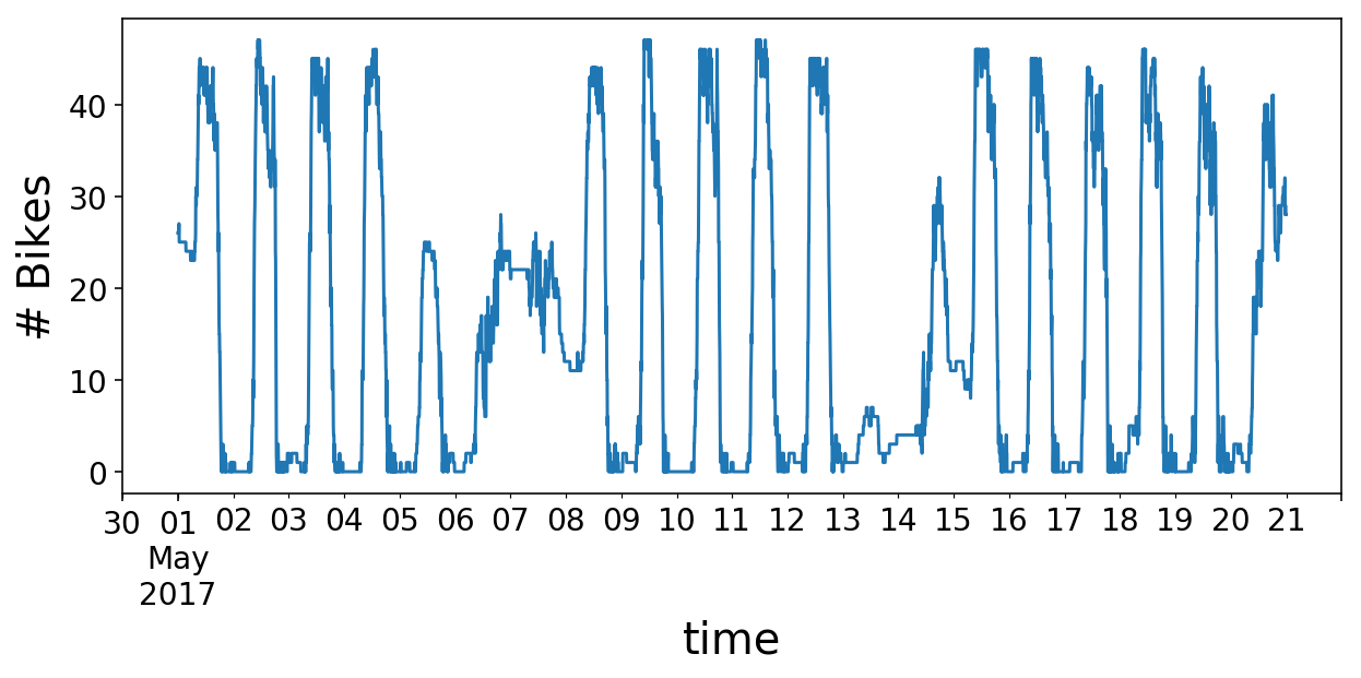
To start out, let’s import some normal libraries and cargo the outdated Citi Bike information. Recall that the information consists of the variety of bikes obtainable at a station as a operate of time. Simply by eye, we are able to see that there’s some every day and weekly periodicity.
%config InlineBackend.figure_format = 'retina' # dogwhistling for 4K peeps

import warnings

import matplotlib as mpl
import matplotlib.pyplot as plt
import numpy as np
import pandas as pd

plt.ion()

mpl.rcParams['axes.labelsize'] = 20
mpl.rcParams['axes.titlesize'] = 24
mpl.rcParams['figure.figsize'] = (8, 4)
mpl.rcParams['xtick.labelsize'] = 14
mpl.rcParams['ytick.labelsize'] = 14
mpl.rcParams['legend.fontsize'] = 14

warnings.filterwarnings('ignore', class=FutureWarning)
# Load and kind the dataframe.
df = pd.read_pickle('home_dat_20160918_20170604.pkl')
df.set_index('last_communication_time', inplace=True)
df.index = pd.to_datetime(df.index)
df.sort_index(inplace=True)

# Select our time collection object
# and repair it to a 5-min sampling interval
y = df.available_bikes
y.index.title = 'time'
y = y.resample('5T').final()
y = y.fillna(technique='ffill')
y.loc['2017-05-01':'2017-05-20'].plot(figsize=(10, 4));
plt.ylabel('# Bikes');
# Convert to an array for the remainder of the submit
y = y.values
Checking Stationarity
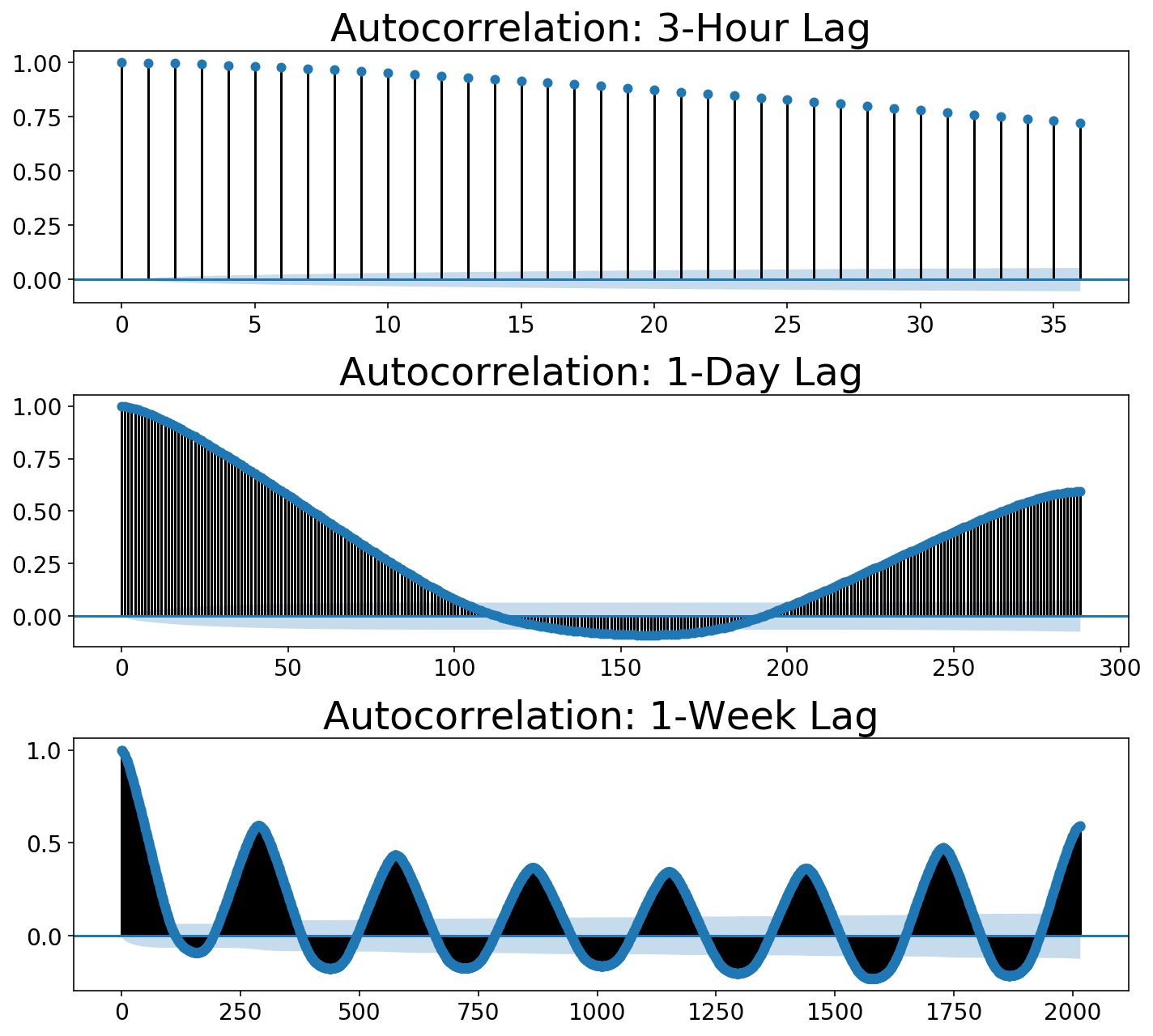
For posterity, let’s stroll by how to take a look at the stationarity of the information (like, within the correct option to estimate ARIMA parameters). The frequent technique of checking to see if information is stationary is to plot its autocorrelation operate. The autocorrelation entails “sliding” or “shifting” a operate and multiplying it with its unshifted self. This enables one to measure the overlap of the operate with itself at completely different deadlines. This course of finally ends up being helpful for locating periodicity in ones information. For instance, a sine wave repeats itself each $2pi$, so one would see peaks within the autocorrelation operate each $2pi$. If that’s complicated, please take a look at this nice submit which incorporates an explanatory animation.
We are able to use statsmodels to plot our autocorrelation operate. We are able to use the autocorrelation operate to quantify this. Beneath, I plot three autocorrelations at completely different numbers of “lags” (the terminology statsmodels makes use of). Our residual samples are 5 minutes aside. Every plot under appears on the autocorrelation going out to a while window or “variety of lags”. Autocorrelations all the time begin at 1 (a operate completely overlaps with itself), however we want to see that it drops down near zero. These plots present that it certaintly doesn’t!
Discover that the autocorrelation rises as we hit 1-day of periodicity within the second plot. Within the third plot, we get every day peaks however a fair larger peak out on the seventh day which corresponds to the weekly periodicity or “seasonality”.
import statsmodels.tsa.api as smt


def plot_multi_acf(information, lags, titles, ylim=None, partial=False):
    num_plots = len(lags)
    fig, ax = plt.subplots(len(lags), 1, figsize=(10, 3 * num_plots));
    if num_plots == 1:
        ax = [ax]
    acf_func = smt.graphics.plot_pacf if partial else smt.graphics.plot_acf
    for idx, (lag, title) in enumerate(zip(lags, titles)):
        fig = acf_func(information, lags=lag, ax=ax[idx], title=title);
        if ylim is not None:
            ax[idx].set_ylim(ylim);

    fig.tight_layout();

period_minutes = 5
samples_per_hour = int(60 / period_minutes)
samples_per_day = int(24 * samples_per_hour)
samples_per_week = int(7 * samples_per_day)

lags = [3 * samples_per_hour, samples_per_day, samples_per_week]
titles= ['Autocorrelation: 3-Hour Lag',
         'Autocorrelation: 1-Day Lag',
         'Autocorrelation: 1-Week Lag']

plot_multi_acf(y, lags, titles)
Reversible Transformations
So we should always in all probability attempt differencing our information. That’s, we should always subtract the adjoining level from every level. This looks like a easy idea. Heaps of posts reference the DataFrame.shift() operate in pandas as a simple option to subtract shifted information. My neurotic concern was that, as soon as one does this, it’s nontrivial to reconstruct the unique time collection. Consequently, how does one then feed the differenced information by a mannequin and plot the prediction alongside the unique information?
Moreover, one performs regression on the distinction time collection information in an ARIMA mannequin. This can be a distinctive downside that reveals the place time collection diverge from standard machine studying through scikit-learn. Whereas one could construct and manipulate a bunch of options for an ML prediction, the goal values (i.e. $y$) are sometimes left alone. I, for one, am all the time scared too contact them lest I leak goal data into my options. With time collection, although, one should truly remodel the y variable that’s fed into the eventual mannequin match(X, y) technique.
Given the wants that I had – reversible transformations and the power to change each X and y – I ended up constructing a library that’s impressed by scikit-learn (all lessons inherit from scikit-learn lessons), however there are undoubtedly untoward actions deviating from the scikit-learn paradigm. As talked about on the prime, this library known as skits, and might be discovered on my github. I ought to warn that it’s undoubtedly a piece in progress with a non-stationary API (har har har).
Why not use an present library?
statsmodels has lots of time collection fashions together with plotting and pandas integrations. Nevertheless, I had problem determining what was happening underneath the hood. Additionally, I didn’t perceive how one would use a educated mannequin on new information. And even when I did determine this out, who the hell is aware of the way you serialize these fashions? Lastly, I just like the composability of scikit-learn. If I wish to throw a neural community on the finish of a pipeline, why shouldn’t I be capable to?
After I began this submit, I discovered this library tsfresh which does seem to permit one to construct options out of time collection and throw them in a scikit-learn pipeline. Nevertheless, this library does so many issues and builds so many options, and I couldn’t determine do something easy with it. It felt like a sledgehammer, and I simply wanted a tapper. Nonetheless, the library appears extraordinarily highly effective, and I’d like to play with it given an appropriate dataset.
I want to name out Fb’s prophet which appears wonderful for understanding uncertainty in time collection predictions. Uncertainty in time collection is usually fairly giant (it’s arduous to foretell the long run!), so quantifying that is typically of paramount significance (assume: threat administration). I want to write about this library in a future submit.
Lastly, I’ll speak later about forecasting, however I’ll say now that I wished the power to construct fashions that immediately optimize for “multi-step forward” forecasting which I’ve not seen extensively applied.
Preprocessing with skits
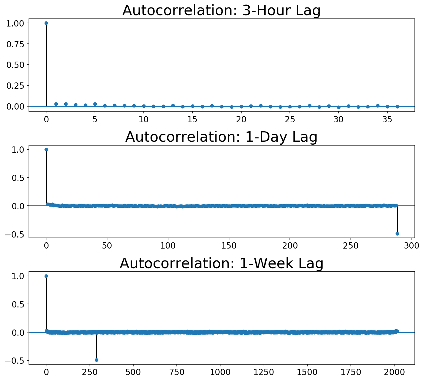
We want to distinction our information and plot the autocorrelation. We are able to use the DifferenceTransformer class in skits to distinction the information. Once we distinction the information, we are going to essentially create some Null (np.nan) values within the information (we can’t subtract the sooner level from the primary level within the array). scikit-learn doesn’t like Null values, so we are going to use a ReversibleImputer to fill in these values. The opposite choice could be to take away the Null values, however the variety of rows in your information by no means adjustments in scikit-learn pipelines, and I didn’t wish to deviate from that habits. Each of those steps happen earlier than we find yourself constructing machine studying options with the information, so they’re within the skits.preprocessing module. All lessons in preprocessing comprise inverse_transform() strategies such that we reconstruct the unique time collection.
We want to chain their transformations collectively, so we are going to use the ForecasterPipeline in skits.pipeline. On account of me not determining a greater means to do that, all preprocessing transformers should prefix their title with 'pre_'.
from skits.preprocessing import (ReversibleImputer,
                                 DifferenceTransformer)
from skits.pipeline import ForecasterPipeline
from sklearn.preprocessing import StandardScaler
We now assemble the pipeline, match the transformers, and remodel the information. Our design matrix, $X$, is only a copy of the $y$ time collection, although we should add an additional axis as a result of scikit-learn expects 2D design matrices. I find yourself needing to make use of two differencing operations with the intention to stationarize the residuals. The primary is a typical differencing operation between adjoining factors. The second differencer handles the seasonality within the information by taking the distinction between factors separated by a day. We additionally want a ReversibleImputer in between every differencing operation to deal with the Null values. A StandardScaler is used on the finish to maintain the information normalized.
pipeline = ForecasterPipeline([
    ('pre_differencer', DifferenceTransformer(period=1)),
    ('pre_diff_imputer', ReversibleImputer()),
    ('pre_day_differencer', DifferenceTransformer(period=samples_per_day)),
    ('pre_day_diff_imputer', ReversibleImputer()),
    ('pre_scaler', StandardScaler())
])

X = y.copy()[:, np.newaxis]

Xt = pipeline.fit_transform(X, y)
As earlier than, we are able to plot the autocorrelation capabilities. You’ll be able to see that the 3-Hour view reveals the autocorrelation instantly dropping to zero, whereas the every day views present that it takes in the future for the autocorrelation to drop to zero.
plot_multi_acf(Xt.squeeze(), lags, titles)
The Field-Jenkins technique requires not solely trying on the autocorrelation operate but additionally the partial autocorrelation:
plot_multi_acf(Xt.squeeze(), lags, ['Partial ' + t for t in titles],
               partial=True)
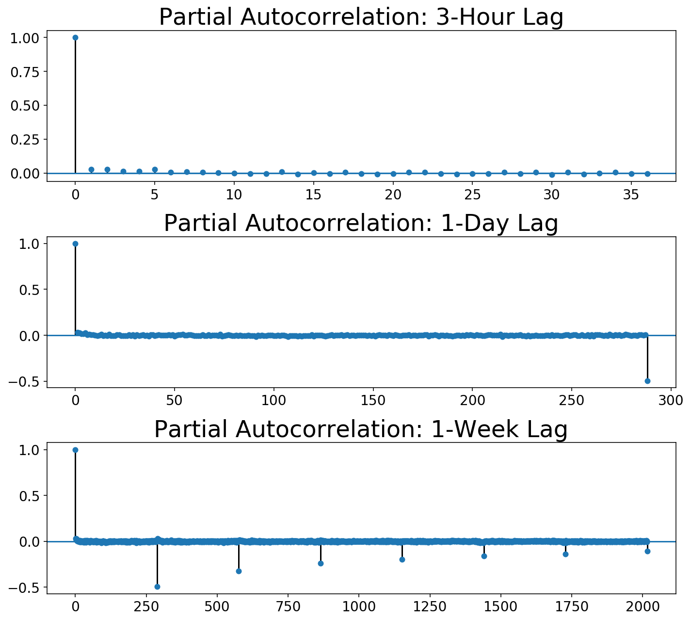
We are able to see that, whereas the autocorrelation drops to zero after in the future lag, the partial autocorrelation slowly decays over day lags. So far as I can inform, Field-Jenkins says that that is probably a seasonal shifting common mannequin. Sadly, we are able to’t do this with our scikit-learn-style framework!
So, let’s transfer on and check out modeling this with autogregressive phrases so I can not less than present you mannequin with skits 🙂
Becoming and Predicting with skits
After preprocessing, we have to construct some options and so as to add on a regression mannequin. We’ll create options akin to a single autoregressive time period and a single seasonal autoregressive time period akin to a lag of a day. All of those options ought to be added after the preprocessing steps through a FeatureUnion. We’ll use linear regression as our regression mannequin.
from skits.pipeline import ForecasterPipeline
from skits.feature_extraction import (AutoregressiveTransformer,
                                      SeasonalTransformer)
from sklearn.linear_model import LinearRegression, LogisticRegression, Ridge
from sklearn.ensemble import (RandomForestClassifier, GradientBoostingClassifier,
                              RandomForestRegressor)
from sklearn.metrics import mean_squared_error
from sklearn.pipeline import FeatureUnion
from sklearn.preprocessing import StandardScaler
pipeline = ForecasterPipeline([
    ('pre_differencer', DifferenceTransformer(period=1)),
    ('pre_diff_imputer', ReversibleImputer()),
    ('pre_day_differencer', DifferenceTransformer(period=samples_per_day)),
    ('pre_day_diff_imputer', ReversibleImputer()),
    ('pre_scaler', StandardScaler()),
    ('features', FeatureUnion([
        ('ar_features', AutoregressiveTransformer(num_lags=1)),
        ('seasonal_features', SeasonalTransformer(seasonal_period=samples_per_day)),
    ])),
    ('post_feature_imputer', ReversibleImputer()),
    ('post_feature_scaler', StandardScaler()),
    ('regressor', LinearRegression(fit_intercept=False))
])

pipeline = pipeline.match(X, y)
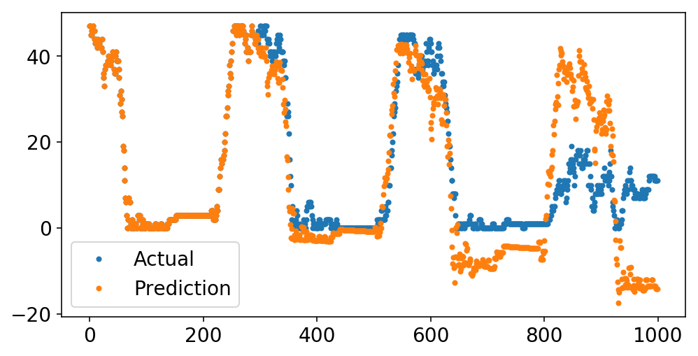
We are able to now plot our predictions alongside the unique information. Recall that every “prediction” level is simply the expected worth of the time collection at that time, given the entire information previous to that time.
Beneath, we predict the final 1000 factors of the collection. Whereas the prediction begins off stable, it shortly begins to veer into loopy land containing issues like detrimental obtainable bikes. I’ve two theories why this occurs:
- We want shifting common phrases.
- Differencing operations are very harmful. As a way to invert the
DifferenceTransformer, we should calculate a cumulative sum. Any small floating level errors will get cumulatively magnified on this course of. Coincidentally, this is the reason numerical integrations are greatest averted, and I suppose now I’m beginning to perceive why these are the Built-in phrases.
plt.plot(y[-1000:], '.');
plt.plot(pipeline.predict(X[-1000:], to_scale=True), '.');
plt.legend(['Actual', 'Prediction']);
What’s terrifying is that I can simplify our pipeline drastically and get a superb match.
pipeline = ForecasterPipeline([
    ('features', FeatureUnion([
        ('ar_features', AutoregressiveTransformer(num_lags=1)),
    ])),
    ('post_feature_imputer', ReversibleImputer()),
    ('regressor', LinearRegression(fit_intercept=False))
])

pipeline = pipeline.match(X, y)
plt.plot(y[-1000:], '.');
plt.plot(pipeline.predict(X[-1000:], to_scale=True), '.');
plt.legend(['Actual', 'Prediction']);
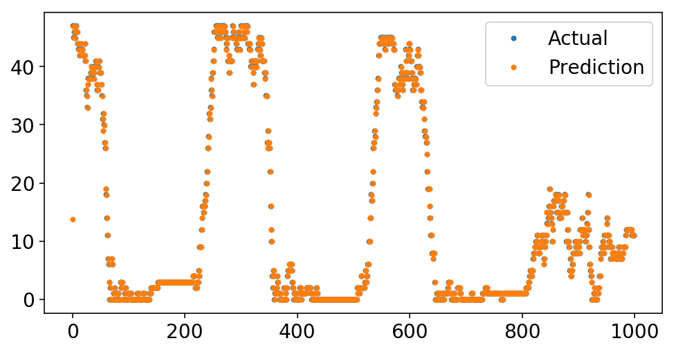
Wow, take a look at that match! And all with solely a single autoregressive time period. What’s happening?
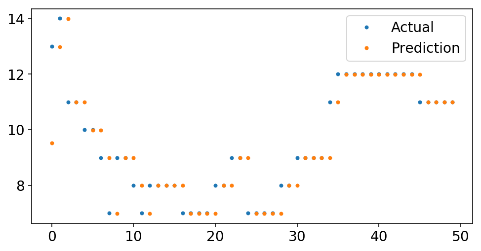
We begin by having a look on the coefficient of the one autoregressive time period:
print(f'Autoregressive Lag Coefficient = {pipeline.named_steps["regressor"].coef_[0]:4.3f}')
Autoregressive Lag Coefficient = 0.999
It’s virtually one. That simply implies that we’re predicting that the subsequent worth would be the final worth. If we glance nearer on the information, we are able to see this eye.
plt.plot(y[-50:], '.');
plt.plot(pipeline.predict(X[-50:], to_scale=True), '.');
plt.legend(['Actual', 'Prediction']);
Forecasting
For the five-minute sampling interval of our information, prediting the final level is the subsequent level might be a good guess. However, has our mannequin truly discovered something?
On one hand, if we wish to accurately guess the variety of bikes obtainable within the subsequent 5 minutes, we’re going to be fairly correct:
mse = mean_squared_error(y, pipeline.predict(X, to_scale=True))
rmse = np.sqrt(mse)
print(f'RMSE = {rmse:4.2f}')
RMSE = 1.13
However, if we had been to feed our mannequin’s prediction as the subsequent level within the collection and proceed to make predictions off the mannequin predictions, our predictions would by no means change. If the previous = the long run, then why ought to something change? This the so known as out of pattern forecasting. We are able to truly do that with skits utilizing the forecast technique. We run in-sample predictions up till the start_idx, after which we begin forecasting.
start_idx = 125

plt.plot(y[-500:], '.');
plt.plot(pipeline.forecast(X[-500:, :], start_idx=start_idx), '.');

ax = plt.gca();
ylim = ax.get_ylim();
plt.plot((start_idx, start_idx), ylim);
plt.ylim(ylim);
plt.legend(['Actual', 'Forecast', 'Forecast Start']);
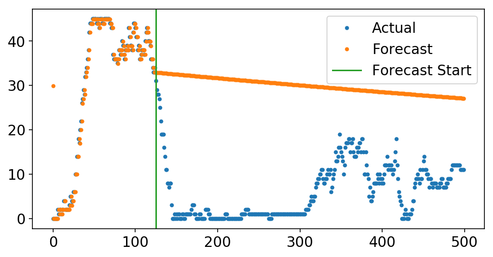
The above is my try to illuminate why easy ARIMA fashions might be useful – I knew what the forecast would seem like earlier than I even plotted it. Realizing how a deterministic course of will play out is, like, the inspiration of a lot of science. Nevertheless, once I consider these fashions from the machine studying facet, they appear foolish. If you’d like your mannequin to forecast nicely, then why not bake that into your loss operate and truly optimize for this? That, my buddies, must watch for the subsequent submit.
Time Sequence Classification
I got down to study time collection in order that I may know if there could be docks obtainable at a future time limit at a Citi Bike station. In any case my waxing and waning above, let’s get again to the true world and apply our data.
For simplicity, let’s resolve the issue of predicting whether or not there will probably be any bikes obtainable on the station. I don’t care precisely what number of bikes are on the station – I simply wish to know if there will probably be any. We are able to thus forged this as a classification downside. I’ll maintain my authentic X matrix containing the variety of bikes, however I’ll flip the y array right into a binary indicator of whether or not or not there are any bikes. We now have an inexpensive quantity of sophistication imbalance, which is nice – there are sometimes bikes!
skits incorporates a ClassificationPipeline which permits one so as to add on a classification mannequin on the finish. One also can management what number of steps out sooner or later they wish to predict. Let’s say that I’m quarter-hour away from a station. We’ll attempt to predict if there will probably be bikes quarter-hour from now, which corresponds to three information factors sooner or later. This time period have to be included in the entire characteristic transformers that depend on earlier values of the information through the pred_stride time period.
from skits.pipeline import ClassifierPipeline
from sklearn.linear_model import LogisticRegression
pipeline = ClassifierPipeline([
    ('features', FeatureUnion([
        ('ar_features', AutoregressiveTransformer(num_lags=1, pred_stride=3)),
    ])),
    ('post_feature_imputer', ReversibleImputer()),
    ('classifier', LogisticRegression(fit_intercept=False))
])

pipeline = pipeline.match(X, y)
y_pred = pipeline.predict_proba(X)[:, 1]
from sklearn.metrics import roc_auc_score
print(f'AUC = {roc_auc_score(y, y_pred):4.2f}')
AUC = 0.98
And so we get superb AUC with solely a single worth of the information quarter-hour earlier. We’re probably solely accurately classifying trivial examples and never getting proper the examples that matter (like when the bikes quickly deplete throughout rush hour). We are able to immediately visualize this by plotting the true variety of bikes alongside the mode’s predicted chance of there being not less than one bike. What you see is that it appears like a scaled model of our earlier, regression plot. This is smart, as a result of that is simply the sooner plot handed by the sigmoid operate of Logisitic Regression.
fig, ax = plt.subplots();
ax.plot(X[-2000:, 0], '.');
ax2 = ax.twinx();
ax2.plot(y_pred[-2000:],
         '.',
         c=ax._get_lines.get_next_color());
ax2.set_ylim((0, 1.1));

ax.set_ylabel('True # Bikes');
ax2.set_ylabel('Likelihood > 0 Bikes');
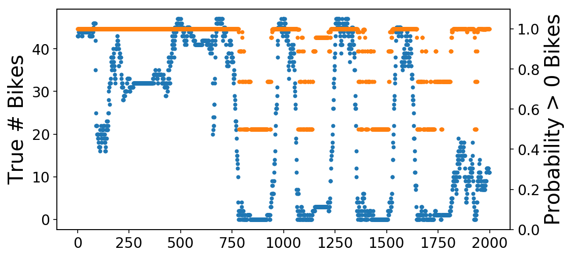
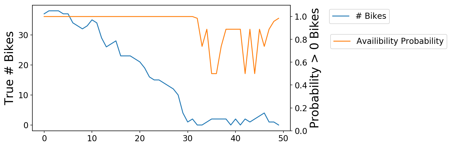
We are able to then zoom in on one of many transitions from obtainable to zero bikes. As you see, the chance (orange) line is gradual to react to those adjustments (although that is admittedly a tough downside).
fig, ax = plt.subplots();
ax.plot(X[-1250:-1200], '-');
ax2 = ax.twinx();
ax2.plot(y_pred[-1250:-1200],
         '-',
         c=ax._get_lines.get_next_color());
ax2.set_ylim((0, 1.1));
ax.set_ylabel('True # Bikes');
ax2.set_ylabel('Likelihood > 0 Bikes');
ax.legend(['# Bikes'], bbox_to_anchor=(1.4, 1));
ax2.legend(['Availibility Probability'], bbox_to_anchor=(1.14, .8));
We are able to strategy assuaging this downside in two methods – we are able to construct out selective coaching information to concentrate on the extra vital examples, or we are able to attempt to construct a correct forecasting mannequin such that we are able to deal with each trivial and nontrivial instances. I’ll concentrate on the latter within the subsequent submit.
