On this put up we’re going to do a bunch of cool issues following up on the final put up introducing implicit matrix factorization. We’re going to discover Studying to Rank, a distinct technique for implicit matrix factorization, after which use the library LightFM to include facet info into our recommender. Subsequent, we’ll use scikit-optimize to be smarter than grid seek for cross validating hyperparameters. Lastly, we’ll see that we are able to transfer past easy user-to-item and item-to-item suggestions now that we have now facet info embedded in the identical area as our customers and objects. Let’s go!
Historical past lesson
Once I began working at Birchbox, I used to be tasked with discovering a method to incorporate our wealthy buyer info into the implicit suggestions matrix factorization advice system. I had no thought what I used to be doing, so I did numerous google looking out. This proved a tough drawback as a result of there are generally two paradigms of recommender methods – content-based approaches, like when one has demographic buyer information and makes use of this information to seek out different related prospects, and “ratings-based” approaches, like when one has information on what every person rated every merchandise they interacted with. The need was for me to marry these two approaches.
Studying by means of the basic survey article, Matrix Factorization Strategies for Recommender Methods (pdf hyperlink), revealed a bit titled “Extra Enter Sources”. This comprises one such strategy to incorporating so-called “facet info” right into a recommender system. The concept was comparatively easy (properly, easy relative to the preliminary hurdle of wrapping one’s head round matrix factorization). Let’s say that in a daily matrix factorization mannequin, a person $u$ is represented by a single vector $textbf{x}_{u}$ containing that person’s latent components (see earlier posts for extra background on this). Now, let’s say that we have now some demographic details about that person like
| Characteristic | Worth |
|---|---|
| gender | Feminine |
| age_bucket | 25-34 |
| income_bucket | $65-79K |
We will one-hot-encode every of those options into an “attribute-space” $A$ and assume that every every attribute $a$ has its personal latent vector $textbf{s}_{a}$. Lastly, we make the belief that our “whole” person vector is the unique person vector $textbf{x}_{u}$ plus every of the related attribute vectors. If $N(u)$ represents the set of attributes that pertain to person $u$, then the entire person vector is
$$textbf{x}_{u} + sumlimits_{a in N(u)}textbf{s}_{a}$$
One could make the identical set of assumptions for facet details about the objects, and now you cannot solely obtain higher outcomes together with your suggestions, however you too can study vectors and consequently similarities between the facet info vectors. For a basic overview of this, see a put up I wrote for Dia&Co’s tech weblog.
Okay, the strategy is evident, so presumably we simply add this to final put up’s implicit suggestions goal operate and resolve, proper? Effectively, I ran the mathematics, and sadly this isn’t scalable. With the additional set of facet info vectors, final put up’s Alternating Least Squares (ALS) turns into a three-way alternating drawback. There was a particular trick in that ALS optimization that exploited the sparsity of the info to scale the computation. Alas, this trick can’t be used through the stage of ALS the place one is fixing for the facet info vectors.
So what to do now?
Studying to Rank – BPR
It seems that there’s one other technique of optimizing implicit suggestions matrix factorization issues which is neither ALS nor typical stochastic gradient descent (SGD) on final put up’s goal operate. This technique of optimization sometimes goes by the title Studying to Rank and originated in info retrieval principle.
A basic technique of utilizing Studying to Rank with implicit suggestions was within the paper BPR: Bayesian Customized Rating from Implicit Suggestions (pdf hyperlink) first-authored by Steffen Rendle who’s form of a badass in all issues implicit and factorized. The concept is centered round sampling constructive and adverse objects and operating pairwise comparisons. Let’s assume that for this instance our dataset consists of the variety of occasions customers have clicked on varied objects on an internet site. BPR proceeds as follows (in simplified type):
- Randomly choose a person $u$ after which choose a random merchandise $i$ which the person has clicked on. That is our constructive merchandise.
- Randomly choose an merchandise $j$ which the person has clicked on $fewer$ occasions than merchandise $i$ (this contains objects that they’ve by no means clicked). That is our adverse merchandise.
- Use no matter equation you wish to predict the “rating”, $p_{ui}$, for person $u$ and constructive merchandise $i$. For matrix factorization, this can be $textbf{x}_{u} cdot textbf{y}_{i}$.
- Predict the rating for person $u$ and adverse merchandise $j$, $p_{uj}$.
- Discover the distinction between the constructive and adverse scores $x_{uij} = p_{ui} – p_{uj}$.
- Go this distinction by means of a sigmoid and use it as a weighting for updating all the mannequin parameters by way of stochastic gradient descent (SGD).
This technique appeared form of radical to me once I first learn it. Notably, we don’t care concerning the precise worth of the rating that we’re predicting. All we care about is that we rank objects which the person has clicked on extra incessantly greater than objects which the person has clicked on fewer occasions. And thus, our mannequin “learns to rank” 🙂
As a result of this mannequin employs a sampling-based strategy, the authors present that it may be fairly quick and scalable relative to different, slower strategies. Moreover, the authors argue that BPR immediately optimizes the world underneath the ROC curve (AUC) which could possibly be a fascinating attribute. Most significantly for me, it permits one to simply add in facet info with out blowing up the computational pace.
Studying to Rank – WARP
A detailed relative of BPR is Weighted Approximate-Rank Pairwise loss (WARP loss) first launched in WSABIE: Scaling Up To Giant Vocabulary Picture Annotation by Weston et. al. WARP is sort of just like BPR: you pattern a constructive and adverse merchandise for a person, predict for each, and take the distinction. In BPR you then make the SGD replace with this distinction as a weight. In WARP, you solely run the SGD replace for those who predict fallacious, i.e. you expect the adverse merchandise has a better rating than the constructive merchandise. If you don’t predict fallacious, you then hold drawing adverse objects till you both get the prediction fallacious or attain some cutoff worth.
The authors of the WARP paper declare that this course of shifts from optimizing AUC in BPR to optimizing the precision @ okay. The appears possible extra related for many recommender methods, and I often have higher luck optimizing WARP loss over BPR loss. WARP does introduce two hyperparameters, although. One is the margin which determines how fallacious your prediction have to be to implement the SGD replace. Within the paper, the margin is 1 that means you could guess $p_{uj} gt p_{ui} + 1$ to implement the SGD replace. The opposite hyperparameter is the cutoff which determines what number of occasions you’re prepared to attract adverse samples making an attempt to get a fallacious prediction earlier than you quit and transfer on to the following person.
This sampling strategy causes WARP to run rapidly when it begins coaching since you simply get predictions fallacious with an untrained mannequin. After coaching, although, WARP will run slower as a result of it has to pattern and predict many objects till it will get a fallacious prediction and may replace. Seems like a constructive drawback if it’s laborious to get your mannequin to foretell fallacious, although.
LightFM
Again to my Birchbox story. I initially carried out BPR with facet info in pure numpy and scipy. This proved to be fairly gradual, and round that point the LightFM package deal was open sourced by the individuals at Lyst. LightFM is written in Cython and is paralellized by way of HOGWILD SGD. This blew my code out of the water, and I fortunately converted to LightFM.
LightFM makes use of the identical technique as above to include facet info – it assumes that the entire “person vector” is the sum of every of the person’s related facet info vectors (which it calls person “options) and treats the objects analogously. Above, we assumed that we had two kinds of latent vectors: $textbf{x}_{u}$ and $textbf{s}_{a}$. LightFM treats every part as facet info, or options. If we wish to have a particular person vector for person $u$, then we should one-hot-encode that as a single characteristic for that person.
Let’s go forward and set up LightFM, learn in our good previous Sketchfab “likes” information in addition to the mannequin tags, and see if we are able to get higher outcomes with LightFM than we did final put up utilizing basic ALS.
Set up
LightFM is on pypi, so you possibly can set up easiest with pip:
In case you are on a mac, then you’ll sadly not be capable of run your code in parallel out of the field. If you want to make use of parallelization, you could first ensure you have gcc which may be put in with brew:
brew set up gcc --without-multilib
Watch out, this takes like half-hour. The only means I’ve then discovered to constructing LightFM is to trick it. First clone the repository
git clone git@github.com:lyst/lightfm.git
Then, open setup.py go to the place the variable use_openmp is outlined, and laborious set it to True. Then, cd lightfm && pip set up -e .
With all that accomplished, let’s write some code to coach some fashions.
Knowledge preprocessing
I took numerous the capabilities used final time for arranging the Sketchfab information right into a matrix and positioned all of them in a helpers.py file within the rec-a-sketch repo.
%matplotlib inline
import matplotlib.pyplot as plt
import numpy as np
import pandas as pd
import scipy.sparse as sp
from scipy.particular import expit
import pickle
import csv
import copy
import itertools
from lightfm import LightFM
import lightfm.analysis
import sys
sys.path.append('../')
import helpers
df = pd.read_csv('../information/model_likes_anon.psv',
                 sep='|', quoting=csv.QUOTE_MINIMAL,
                 quotechar='')
df.drop_duplicates(inplace=True)
df.head()
| modelname | mid | uid | |
|---|---|---|---|
| 0 | 3D fanart Noel From Sora no Methodology | 5dcebcfaedbd4e7b8a27bd1ae55f1ac3 | 7ac1b40648fff523d7220a5d07b04d9b |
| 1 | 3D fanart Noel From Sora no Methodology | 5dcebcfaedbd4e7b8a27bd1ae55f1ac3 | 2b4ad286afe3369d39f1bb7aa2528bc7 |
| 2 | 3D fanart Noel From Sora no Methodology | 5dcebcfaedbd4e7b8a27bd1ae55f1ac3 | 1bf0993ebab175a896ac8003bed91b4b |
| 3 | 3D fanart Noel From Sora no Methodology | 5dcebcfaedbd4e7b8a27bd1ae55f1ac3 | 6484211de8b9a023a7d9ab1641d22e7c |
| 4 | 3D fanart Noel From Sora no Methodology | 5dcebcfaedbd4e7b8a27bd1ae55f1ac3 | 1109ee298494fbd192e27878432c718a |
# Threshold information to solely embody customers and fashions with min 5 likes.
df = helpers.threshold_interactions_df(df, 'uid', 'mid', 5, 5)
Beginning interactions information
Variety of rows: 62583
Variety of cols: 28806
Sparsity: 0.035%
Ending interactions information
Variety of rows: 15274
Variety of columns: 25655
Sparsity: 0.140%
# Go from dataframe to likes matrix
# Additionally, construct index to ID mappers.
likes, uid_to_idx, idx_to_uid,
mid_to_idx, idx_to_mid = helpers.df_to_matrix(df, 'uid', 'mid')

likes
<15274x25655 sparse matrix of kind '<class 'numpy.float64'>'
    with 547477 saved components in Compressed Sparse Row format>
practice, check, user_index = helpers.train_test_split(likes, 5, fraction=0.2)
The one odd factor that we should do which is completely different than final time is to repeat the coaching information to solely embody customers with information within the check set. This is because of utilizing LightFM’s built-in precision_at_k operate versus our hand-rolled one final time and isn’t notably fascinating.
eval_train = practice.copy()
non_eval_users = checklist(set(vary(practice.form[0])) - set(user_index))

eval_train = eval_train.tolil()
for u in non_eval_users:
    eval_train[u, :] = 0.0
eval_train = eval_train.tocsr()
Now we wish to one-hot-encode all the facet info that we have now concerning the Sketchfab fashions. Recall that this info included classes and tags related to every mannequin. The only means I’ve discovered to go about encoding this info is to make use of scikit-learn’s DictVectorizer class. The DictVectorizer takes in a listing of dictionaries the place the dictionaries include options names as keys and weights as values. Right here, we’ll assume that every weight is 1, and we’ll take the important thing to be the mix of the tag kind and worth.
sideinfo = pd.read_csv('../information/model_feats.psv',
                       sep='|', quoting=csv.QUOTE_MINIMAL,
                       quotechar='')
sideinfo.head()
| mid | kind | worth | |
|---|---|---|---|
| 0 | 5dcebcfaedbd4e7b8a27bd1ae55f1ac3 | class | Characters |
| 1 | 5dcebcfaedbd4e7b8a27bd1ae55f1ac3 | class | Gaming |
| 2 | 5dcebcfaedbd4e7b8a27bd1ae55f1ac3 | tag | 3dsmax |
| 3 | 5dcebcfaedbd4e7b8a27bd1ae55f1ac3 | tag | noel |
| 4 | 5dcebcfaedbd4e7b8a27bd1ae55f1ac3 | tag | loli |
# There's in all probability a flowery pandas groupby method to do
# this however I could not determine it out :(

# Construct checklist of dictionaries containing options
# and weights in identical order as idx_to_mid prescribes.
feat_dlist = [{} for _ in idx_to_mid]
for idx, row in sideinfo.iterrows():
    feat_key = '{}_{}'.format(row.kind, str(row.worth).decrease())
    idx = mid_to_idx.get(row.mid)
    if idx is not None:
        feat_dlist[idx][feat_key] = 1
{'category_characters': 1,
 'category_gaming': 1,
 'tag_3d': 1,
 'tag_3dcellshade': 1,
 'tag_3dsmax': 1,
 'tag_anime': 1,
 'tag_girl': 1,
 'tag_loli': 1,
 'tag_noel': 1,
 'tag_soranomethod': 1}
from sklearn.feature_extraction import DictVectorizer
dv = DictVectorizer()
item_features = dv.fit_transform(feat_dlist)
<25655x20352 sparse matrix of kind '<class 'numpy.float64'>'
    with 161510 saved components in Compressed Sparse Row format>
We at the moment are left with an item_features matrix the place every row is a singular merchandise (in the identical order because the columns of the likes matrix), and every column is a singular tag. It seems to be like there are 20352 distinctive tags!
Coaching
Let’s attempt a easy WARP run on LightFM utilizing the default settings and ignoring the merchandise options to start out. I’m solely going to deal with WARP right this moment, as I’ve by no means had a lot luck with BPR. I’ll create a small operate to calculate the educational curve.
def print_log(row, header=False, spacing=12):
    prime = ''
    center = ''
    backside = ''
    for r in row:
        prime += '+{}'.format('-'*spacing)
        if isinstance(r, str):
            center += '| {0:^{1}} '.format(r, spacing-2)
        elif isinstance(r, int):
            center += '| {0:^{1}} '.format(r, spacing-2)
        elif (isinstance(r, float)
              or isinstance(r, np.float32)
              or isinstance(r, np.float64)):
            center += '| {0:^{1}.5f} '.format(r, spacing-2)
        backside += '+{}'.format('='*spacing)
    prime += '+'
    center += '|'
    backside += '+'
    if header:
        print(prime)
        print(center)
        print(backside)
    else:
        print(center)
        print(prime)

def patk_learning_curve(mannequin, practice, check, eval_train,
                        iterarray, user_features=None,
                        item_features=None, okay=5,
                        **fit_params):
    old_epoch = 0
    train_patk = []
    test_patk = []
    headers = ['Epoch', 'train p@5', 'test p@5']
    print_log(headers, header=True)
    for epoch in iterarray:
        extra = epoch - old_epoch
        mannequin.fit_partial(practice, user_features=user_features,
                          item_features=item_features,
                          epochs=extra, **fit_params)
        this_test = lightfm.analysis.precision_at_k(mannequin, check, train_interactions=None, okay=okay)
        this_train = lightfm.analysis.precision_at_k(mannequin, eval_train, train_interactions=None, okay=okay)

        train_patk.append(np.imply(this_train))
        test_patk.append(np.imply(this_test))
        row = [epoch, train_patk[-1], test_patk[-1]]
        print_log(row)
    return mannequin, train_patk, test_patk
mannequin = LightFM(loss='warp', random_state=2016)
# Initialize mannequin.
mannequin.match(practice, epochs=0);

iterarray = vary(10, 110, 10)

mannequin, train_patk, test_patk = patk_learning_curve(
    mannequin, practice, check, eval_train, iterarray, okay=5, **{'num_threads': 4}
)
+------------+------------+------------+
|   Epoch    | practice p@5  |  check p@5  |
+============+============+============+
|     10     |  0.14303   |  0.02541   |
+------------+------------+------------+
|     20     |  0.16267   |  0.02947   |
+------------+------------+------------+
|     30     |  0.16876   |  0.03183   |
+------------+------------+------------+
|     40     |  0.17282   |  0.03294   |
+------------+------------+------------+
|     50     |  0.17701   |  0.03333   |
+------------+------------+------------+
|     60     |  0.17872   |  0.03287   |
+------------+------------+------------+
|     70     |  0.17583   |  0.03333   |
+------------+------------+------------+
|     80     |  0.17793   |  0.03386   |
+------------+------------+------------+
|     90     |  0.17479   |  0.03392   |
+------------+------------+------------+
|    100     |  0.17656   |  0.03301   |
+------------+------------+------------+
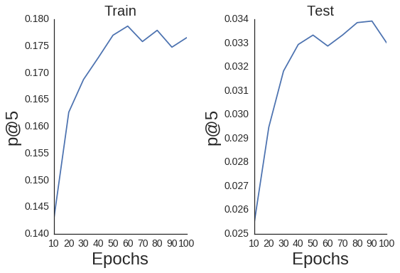
import seaborn as sns
sns.set_style('white')

def plot_patk(iterarray, patk,
              title, okay=5):
    plt.plot(iterarray, patk);
    plt.title(title, fontsize=20);
    plt.xlabel('Epochs', fontsize=24);
    plt.ylabel('p@{}'.format(okay), fontsize=24);
    plt.xticks(fontsize=14);
    plt.yticks(fontsize=14);

# Plot practice on left
ax = plt.subplot(1, 2, 1)
fig = ax.get_figure();
sns.despine(fig);
plot_patk(iterarray, train_patk,
         'Prepare', okay=5)

# Plot check on proper
ax = plt.subplot(1, 2, 2)
fig = ax.get_figure();
sns.despine(fig);
plot_patk(iterarray, test_patk,
         'Check', okay=5)

plt.tight_layout();
Optimizing Hyperparameters with scikit-optimize
Now that we have now a baseline, we want to discover optimum hyperparameters to maximise our p@okay. On a facet be aware, I’m unsure if precision at okay is the perfect metric to be utilizing right here when all of our interactions are binary, however let’s simply ignore that for now…
Final put up I ran a grid search over a bunch of hyperparameters, and it took perpetually. It’s been proven {that a} randomized search is best than express grid search, however we are able to do even higher. Utilizing the scikit-optimize (skopt) library, we are able to deal with the hyperpameters as free parameters to look over whereas utilizing a black field optimization algorithm to maximise p@okay. There are a selection of optimization algorithms to choose from, however I’ll simply follow forest_minimize right this moment.
The setup is fairly easy. You should first outline an goal operate that you simply wish to reduce. The target receives the parameters that you simply wish to resolve for because the arguments and returns the target worth at these parameters. Thus, for our case, we go within the hyperparameters, we practice the LightFM mannequin with these parameters, after which return the p@okay evaluated after coaching. Importantly, we should return the adverse of the p@okay as a result of the target have to be minimized, so maximizing p@okay is identical as minimizing the adverse of the p@okay. The very last thing to notice is that one should make liberal use of world variables as a result of one can solely go hyperparameters to the target operate.
from skopt import forest_minimize
def goal(params):
    # unpack
    epochs, learning_rate,
    no_components, alpha = params

    user_alpha = alpha
    item_alpha = alpha
    mannequin = LightFM(loss='warp',
                    random_state=2016,
                    learning_rate=learning_rate,
                    no_components=no_components,
                    user_alpha=user_alpha,
                    item_alpha=item_alpha)
    mannequin.match(practice, epochs=epochs,
              num_threads=4, verbose=True)

    patks = lightfm.analysis.precision_at_k(mannequin, check,
                                              train_interactions=None,
                                              okay=5, num_threads=4)
    mapatk = np.imply(patks)
    # Make adverse as a result of we wish to _minimize_ goal
    out = -mapatk
    # Deal with some bizarre numerical shit occurring
    if np.abs(out + 1) < 0.01 or out < -1.0:
        return 0.0
    else:
        return out
With the target operate outlined, we are able to outline ranges for our hyperparameters. These can both be easy max and minutes or we are able to assume a distribution like beneath. With the ranges outlined, we easy name forest_minimize and wait a reasonably very long time.
area = [(1, 260), # epochs
         (10**-4, 1.0, 'log-uniform'), # learning_rate
         (20, 200), # no_components
         (10**-6, 10**-1, 'log-uniform'), # alpha
        ]

res_fm = forest_minimize(goal, area, n_calls=250,
                     random_state=0,
                     verbose=True)
print('Maximimum p@okay discovered: {:6.5f}'.format(-res_fm.enjoyable))
print('Optimum parameters:')
params = ['epochs', 'learning_rate', 'no_components', 'alpha']
for (p, x_) in zip(params, res_fm.x):
    print('{}: {}'.format(p, x_))
Maximimum p@okay discovered: 0.04781
Optimum parameters:
epochs: 168
learning_rate: 0.09126423099690231
no_components: 104
alpha: 0.00023540795300720628
No too shabby! We began with a p@okay of ~0.034 with base hyperparameters, after which elevated it to 0.0478 by discovering higher ones. Let’s see what occurs if we add in our merchandise options as facet info to the matrix factorization mannequin.
Studying to Rank + Aspect Data
LightFM makes sure refined assumptions while you do or don’t go facet info. When no user_features or item_features are explicitly included, then LightFM assumes that each characteristic matrices are in reality id matrices of dimension (num_users X num_users) or (num_items X num_items) for person and merchandise characteristic matrices, respectively. What that is successfully doing is one-hot-encoding every person and merchandise ID as a single characteristic vector. Within the case the place you do go an item_features matrix, then LightFM doesn’t do any one-hot-encoding. Thus, every person and merchandise ID doesn’t get its personal vector except you explicitly outline one. The best means to do that is to make your individual id matrix and stack it on the facet of the item_features matrix that we already created. This fashion, every merchandise is described by a single vector for its distinctive ID after which a set of vectors for every of its tags.
# Must hstack item_features
eye = sp.eye(item_features.form[0], item_features.form[0]).tocsr()
item_features_concat = sp.hstack((eye, item_features))
item_features_concat = item_features_concat.tocsr().astype(np.float32)
We now have to outline a brand new goal operate that includes the item_features.
def objective_wsideinfo(params):
    # unpack
    epochs, learning_rate,
    no_components, item_alpha,
    scale = params

    user_alpha = item_alpha * scale
    mannequin = LightFM(loss='warp',
                    random_state=2016,
                    learning_rate=learning_rate,
                    no_components=no_components,
                    user_alpha=user_alpha,
                    item_alpha=item_alpha)
    mannequin.match(practice, epochs=epochs,
              item_features=item_features_concat,
              num_threads=4, verbose=True)

    patks = lightfm.analysis.precision_at_k(mannequin, check,
                                              item_features=item_features_concat,
                                              train_interactions=None,
                                              okay=5, num_threads=3)
    mapatk = np.imply(patks)
    # Make adverse as a result of we wish to _minimize_ goal
    out = -mapatk
    # Bizarre shit occurring
    if np.abs(out + 1) < 0.01 or out < -1.0:
        return 0.0
    else:
        return out
With that outlined, let’s now run a brand new hyperparameter search. I’ll add an additional scaling parameter which is able to management the scaling between the person and merchandise merchandise regularization (alpha) phrases. Due to all the further merchandise options, we could wish to regularize issues otherwise. We’ll additionally enter an x0 time period to forest_minimization which is able to enable us to start out our hyperparameter search on the optimum parameters from the earlier run with out facet info.
area = [(1, 260), # epochs
         (10**-3, 1.0, 'log-uniform'), # learning_rate
         (20, 200), # no_components
         (10**-5, 10**-3, 'log-uniform'), # item_alpha
         (0.001, 1., 'log-uniform') # user_scaling
        ]
x0 = res_fm.x.append(1.)
# This typecast is required
item_features = item_features.astype(np.float32)
res_fm_itemfeat = forest_minimize(objective_wsideinfo, area, n_calls=50,
                                  x0=x0,
                                  random_state=0,
                                  verbose=True)
print('Maximimum p@okay discovered: {:6.5f}'.format(-res_fm_itemfeat.enjoyable))
print('Optimum parameters:')
params = ['epochs', 'learning_rate', 'no_components', 'item_alpha', 'scaling']
for (p, x_) in zip(params, res_fm_itemfeat.x):
    print('{}: {}'.format(p, x_))
Maximimum p@okay discovered: 0.04610
Optimum parameters:
epochs: 192
learning_rate: 0.06676184785227865
no_components: 86
item_alpha: 0.0005563892936299544
scaling: 0.6960826359109953
Now, you is perhaps considering “Ethan, we went by means of all that solely to get worse p@okay?!”, and, frankly, I share your frustration. I’ve truly seen this occur earlier than – including facet info will typically scale back or not less than not enhance no matter metric you’re on the lookout for. In all equity, I solely ran the above optimization for 50 calls, versus the unique one with 250 calls. This was primarily as a result of matrix factorization mannequin operating a lot slower as a result of scaling with the variety of person and merchandise options.
Even so, there are different causes that the outcomes could possibly be worse. Possibly person habits is a a lot better sign than human-defined tags and classes. The tag info could possibly be poor for a number of the fashions. As properly, one could have to scale the tags otherwise in comparison with the distinctive ID vectors utilizing, say, separate regularization phrases, so as to get higher habits. Possibly one ought to normalize the tag weights by the variety of tags. Possibly tags shouldn’t be included except they’ve been used on not less than X fashions. Possibly tags ought to solely be included on fashions with few person interactions as a result of after that ponit the chilly begin drawback is sufficiently null. Who is aware of?! These are experiments I’d like to run, however I’d be joyful to listen to from others’ expertise.
Enjoyable with Characteristic Embeddings
No matter all of this, there’s nonetheless a profit to incorporating the merchandise options. As a result of they’ve vectors embedded in the identical area because the customers and objects, we are able to play with various kinds of suggestions. We’ll first retrain the mannequin on the complete dataset utilizing the optimum parameters.
epochs, learning_rate,
no_components, item_alpha,
scale = res_fm_itemfeat.x

user_alpha = item_alpha * scale
mannequin = LightFM(loss='warp',
                random_state=2016,
                learning_rate=learning_rate,
                no_components=no_components,
                user_alpha=user_alpha,
                item_alpha=item_alpha)
mannequin.match(likes, epochs=epochs,
          item_features=item_features_concat,
          num_threads=4)
Characteristic Sorting
Think about you’re on Sketchfab and click on the tag tiltbrush which might presumably correspond to fashions created with Google’s Tilt Brush VR appliction. How ought to Sketchfab return the outcomes to you? They at present return outcomes based mostly on the recognition of the objects which is presumably not related to the “tiltbrushiness” of the fashions. With the factorized tags, we are able to now return a listing of merchandise which might be most related to the tiltbrush tag sorted by that similarity. To do that, we should discover the tiltbrush vector and measure the cosine similarity to each product.
Recall that we tacked our id matrix onto the left-hand facet of the item_features matrix. Which means that our DictVectorizer, which mapped our merchandise options to column indices of our item_features matrix, may have indices which might be off by the variety of objects.
idx = dv.vocabulary_['tag_tiltbrush'] + item_features.form[0]
Subsequent, we have to calculate the cosine similarity between the tiltbrush vector and all different merchandise representations the place every merchandise’s illustration is the sum of its characteristic vectors. These characteristic vectors are saved as item_embeddings within the LightFM mannequin. (Be aware: there are technically bias phrases within the LightFM mannequin that we’re merely ignoring for now).
def cosine_similarity(vec, mat):
    sim = vec.dot(mat.T)
    matnorm = np.linalg.norm(mat, axis=1)
    vecnorm = np.linalg.norm(vec)
    return np.squeeze(sim / matnorm / vecnorm)

tilt_vec = mannequin.item_embeddings[[idx], :]
item_representations = item_features_concat.dot(mannequin.item_embeddings)
sims = cosine_similarity(tilt_vec, item_representations)
Lastly, we are able to repurpose some code from the final weblog put up to visualise the highest 5 Sketchfab mannequin thumbnails which might be most just like the tiltbrush vector.
import requests
def get_thumbnails(row, idx_to_mid, N=10):
    thumbs = []
    mids = []
    for x in np.argsort(-row)[:N]:
        response = requests.get('https://sketchfab.com/i/fashions/{}'
                                .format(idx_to_mid[x])).json()
        thumb = [x['url'] for x in response['thumbnails']['images']
                 if x['width'] == 200 and x['height']==200]
        if not thumb:
            print('no thumbnail')
        else:
            thumb = thumb[0]
        thumbs.append(thumb)
        mids.append(idx_to_mid[x])
    return thumbs, mids
from IPython.show import show, HTML

def display_thumbs(thumbs, mids, N=5):
    thumb_html = "<a href='{}' goal='_blank'>
                  <img type='width: 160px; margin: 0px;
                  border: 1px stable black;'
                  src='{}' /></a>"
    pictures = ''
    for url, mid in zip(thumbs[0:N], mids[0:N]):
        hyperlink = 'http://sketchfab.com/fashions/{}'.format(mid)
        pictures += thumb_html.format(hyperlink, url)
    show(HTML(pictures))
Fairly cool! Seems like every of those are made with Tiltbrush. Be at liberty to click on the above pictures to take a look at every mannequin on the Sketchfab web site.
What else can we do?
Tag Recommendations
Let’s say that Sketchfab want to encourage individuals to make use of extra tags. That is advantageous to the corporate as a result of it get customers to create structured information for them without spending a dime whereas partaking the person. Sketchfab might encourage this habits by suggesting tags to go together with a picture. A method we might do that can be to take a mannequin and recommend tags to go together with it that aren’t at present there. This entails discovering tag vectors which might be most just like the mannequin after which filtering tags which might be already current.
idx = 900
mid = idx_to_mid[idx]
def display_single(mid):
    """Show thumbnail for a single mannequin"""
    response = requests.get('https://sketchfab.com/i/fashions/{}'
                            .format(mid)).json()
    thumb = [x['url'] for x in response['thumbnails']['images']
             if x['width'] == 200 and x['height']==200][0]
    thumb_html = "<a href='{}' goal='_blank'>
                  <img type='width: 200px; margin: 0px;
                  border: 1px stable black;'
                  src='{}' /></a>"
    hyperlink = 'http://sketchfab.com/fashions/{}'.format(mid)
    show(HTML(thumb_html.format(hyperlink, thumb)))

display_single(mid)

# Make mapper to map from from characteristic index to characteristic title
idx_to_feat = {v: okay for (okay, v) in dv.vocabulary_.objects()}
print('Tags:')
for i in item_features.getrow(idx).indices:
    print('- {}'.format(idx_to_feat[i]))

Tags:
- category_architecture
- category_characters
- category_cultural heritage
- category_products & know-how
- category_science, nature & training
- tag_rock
- tag_sculpture
- tag_woman
# Indices of all tag vectors
tag_indices = set(v for (okay, v) in dv.vocabulary_.objects()
                  if okay.startswith('tag_'))
# Tags which might be already current
filter_tags = set(i for i in item_features.getrow(idx).indices)

item_representation = item_features_concat[idx, :].dot(mannequin.item_embeddings)
sims = cosine_similarity(item_representation, mannequin.item_embeddings)

suggested_tags = []
i = 0
recs = np.argsort(-sims)
n_items = item_features.form[0]
whereas len(suggested_tags) < 10:
    offset_idx = recs[i] - n_items
    if offset_idx in tag_indices
       and offset_idx not in filter_tags:
        suggested_tags.append(idx_to_feat[offset_idx])
    i += 1
print('Recommended Tags:')
for t in suggested_tags:
    print('- {}'.format(t))
Recommended Tags:
- tag_greek
- tag_castel
- tag_santangelo
- tag_eros
- tag_humanti
- tag_galleria
- tag_batholith
- tag_rome
- tag_substanced880
- tag_roman
Fast conclusion
So this put up was lengthy. There was rather a lot to study and numerous parameters to optimize. I’d like to notice that, by way of out of the field efficiency, it’s laborious to beat the ALS mannequin from final put up. There’s fewer parameters to optimize, and the mannequin is way more “forgiving” of being a bit off in your hyperparameters. Contrastingly, in case your studying price is poor, then SGD provides you with nothing in return. It’s undoubtedly potential to beat ALS in efficiency, although, for those who spend sufficient time fiddling round. Furthermore, the flexibility to include facet info is essential for with the ability to make new kinds of suggestions and overcome the chilly begin drawback, so it’s good to have this in your toolbox.
