After I first began to find out about machine studying, particularly supervised studying, I ultimately felt snug with taking some enter $mathbf{X}$, and figuring out a operate $f(mathbf{X})$ that finest maps $mathbf{X}$ to some recognized output worth $y$. Individually, I dove a little bit into time sequence evaluation and considered this as a very completely different paradigm. In time sequence, we don’t consider issues when it comes to options or inputs; reasonably, we’ve the time sequence $y$, and $y$ alone, and we take a look at earlier values of $y$ to foretell future values of $y$.
Nonetheless, I usually puzzled, “The place does machine studying finish and time sequence start?”. Or, “How do I exploit “options” in time sequence?”. I suppose when you can reply these questions rather well, then you definitely’re in for making some cash in finance. Or not. I don’t know – I actually know nothing about that world.
I’ve had bother answering these questions, in no small half as a result of frequent problem of coping with domain-specific vocabulary. I discover myself having to internally translate time sequence ideas into “acquainted” machine studying ideas. With this in thoughts, I’d thus wish to kick off a sequence of weblog posts round analyzing time sequence knowledge with the hopes of presenting these ideas in a well-recognized kind. Because of the ubiquity of scikit-learn, I’ll assume that the scikit-learn API constitutes a well-recognized kind.
To start out the sequence off, on this submit I’ll introduce a time sequence dataset that I’ve gathered. I’ll then stroll by means of how we will flip the time sequence forecasting drawback right into a basic linear regression drawback.
Let’s discover a y(t)
The necessities for an acceptable time sequence dataset are pretty minimal: We want some amount that adjustments with time. Ideally, our knowledge set may exhibit some patterns such that we will study some issues like seasonality and cyclic habits. Fortunately, I’ve acquired simply the dataset!
That is the place you groan as a result of I say that the dataset is expounded to the Citi Bike NYC bikeshare knowledge. All people writes about this rattling dataset, and it’s been overwhelmed to demise. Properly, I agree, however hear me out. I’m not utilizing the similar dataset that everyone else makes use of. The everyday Citi Bike dataset consists of all journeys taken on the bikes. My dataset seems to be on the the variety of bikes at every station as a operate of time. Eh?
I began gathering this knowledge a few 12 months and a half in the past as a result of I used to be coping with a typical, irritating situation. I’d test the Citi Bike app to make it possible for there could be docks obtainable on the station by my workplace earlier than I left my residence within the morning. Nonetheless, by the point I rode to the workplace station, all of the docks would have stuffed up, and I’d then have to search around for a special station at which to dock the bike. Ideally, my app ought to inform me that, though there are 5 docks obtainable proper now, they are going to probably be unavailable by the point I get there.
I needed to gather this knowledge and predict this myself. I nonetheless haven’t performed that, however hopefully we are going to in a while on this weblog sequence. Within the meantime, since 9/18/2016, I pinged the Citi Bike API each 2 minutes to gather what number of bikes and docks can be found at each single citi bike station in NYC. Within the spirit of not planning forward, this all simply runs on a cron job on a t2.micro EC2 occasion backed by a Postgres database that’s working regionally on the identical occasion. There are some gaps within the knowledge as a consequence of me sometimes working out of onerous drive house on the occasion. The code for this lives in this repo, and I’ve saved greater than 200 million information.
For extra details about this dataset, I wrote a quick submit on Making Dia.
For our functions as we speak, I’m going to concentrate on a single time sequence from this knowledge. The time sequence consists of the variety of obtainable bikes on the station at East sixteenth St and fifth Ave (i.e. the closest one to my residence) as a operate of time. Particularly, time is listed by the last_communication_time. The Citi Bike API appears to replace its values with random periodicity for various stations. The last_communication_time corresponds to the final time that the Citi Bike API talked to the station on the time of me querying.
We’ll begin by studying the information in with pandas. Pandas might be the popular library to make use of for exploring time sequence knowledge in Python. It was initially constructed for analyzing monetary knowledge which is why it shines so effectively for time sequence. For a superb useful resource on time sequence modeling in pandas, try Tom Aguspurger’s submit in his Trendy Pandas sequence. Whereas I discovered that submit to be extraordinarily useful, I’m extra fascinated by why one does sure issues with time sequence versus how to do these items.
My bike availability time sequence is within the type of a pandas Sequence object and is saved as a pickle file. Usually, one doesn’t care concerning the order of the index in Pandas objects, however, for time sequence, you’ll want to kind the values in chronological order. Be aware that I ensure the index is a sorted pandas DatetimeIndex.
%config InlineBackend.figure_format = 'retina'

import datetime
import time

import matplotlib as mpl
import matplotlib.pyplot as plt
import numpy as np
import pandas as pd

plt.ion()

mpl.rcParams['axes.labelsize'] = 20
mpl.rcParams['axes.titlesize'] = 24
mpl.rcParams['figure.figsize'] = (8, 4)
mpl.rcParams['xtick.labelsize'] = 14
mpl.rcParams['ytick.labelsize'] = 14
mpl.rcParams['legend.fontsize'] = 14
# Load and type the dataframe.

df = pd.read_pickle('home_dat_20160918_20170604.pkl')
df.set_index('last_communication_time', inplace=True)
df.index = pd.to_datetime(df.index)
df.sort_index(inplace=True)
df.head()
| execution_time | available_bikes | available_docks | id | lat | lon | st_address | station_name | status_key | status_value | test_station | total_docks | |
|---|---|---|---|---|---|---|---|---|---|---|---|---|
| last_communication_time | ||||||||||||
| 2016-09-18 16:58:36 | 2016-09-18 16:59:51 | 4 | 43 | 496 | 40.737262 | -73.99239 | E 16 St & 5 Ave | E 16 St & 5 Ave | 1 | In Service | f | 47 |
| 2016-09-18 16:58:36 | 2016-09-18 17:01:47 | 4 | 43 | 496 | 40.737262 | -73.99239 | E 16 St & 5 Ave | E 16 St & 5 Ave | 1 | In Service | f | 47 |
| 2016-09-18 17:02:29 | 2016-09-18 17:03:42 | 7 | 40 | 496 | 40.737262 | -73.99239 | E 16 St & 5 Ave | E 16 St & 5 Ave | 1 | In Service | f | 47 |
| 2016-09-18 17:02:29 | 2016-09-18 17:05:48 | 7 | 40 | 496 | 40.737262 | -73.99239 | E 16 St & 5 Ave | E 16 St & 5 Ave | 1 | In Service | f | 47 |
| 2016-09-18 17:07:06 | 2016-09-18 17:07:44 | 7 | 40 | 496 | 40.737262 | -73.99239 | E 16 St & 5 Ave | E 16 St & 5 Ave | 1 | In Service | f | 47 |
# Select our time sequence object
# and repair it to a 5-min sampling interval

y = df.available_bikes
y.index.title = 'time'
y = y.resample('5T').final()
y.head()
time
2016-09-18 16:55:00     4.0
2016-09-18 17:00:00     7.0
2016-09-18 17:05:00     6.0
2016-09-18 17:10:00     5.0
2016-09-18 17:15:00    10.0
Freq: 5T, Identify: available_bikes, dtype: float64
ax = y.plot();
ax.set_ylabel('# Bikes');
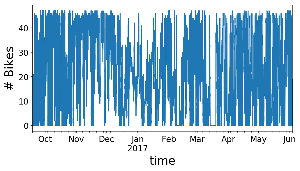
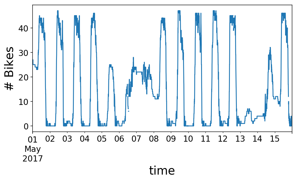
As you’ll be able to see, our time sequence seems to be like type of a large number. We will zoom in on the primary half of Might to get a greater view of what’s occurring. It seems to be like we’ve an everyday rise and fall of our obtainable bikes that occurs every day with considerably completely different habits on the weekends (5/1 was a Monday, and 5/6 was a Saturday, in case you’re questioning).
y.loc['2017-05-01':'2017-05-15'].plot();
plt.ylabel('# Bikes');
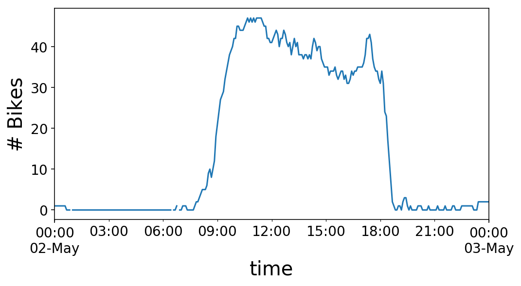
If we zoom in on a single day, we see that the variety of bikes on the station rises within the morning, round 9 AM, after which plummets within the night, round 6 PM. I’d name this a “commuter” station. There are loads of workplaces round this station, so many individuals experience to the station within the morning, drop a motorbike off, after which decide up a motorbike within the night and experience away. This works out completely for me, as I get to take the reverse commute.
y.loc['2017-05-02 00:00:00':'2017-05-03 00:00:00'].plot();
plt.ylabel('# Bikes');
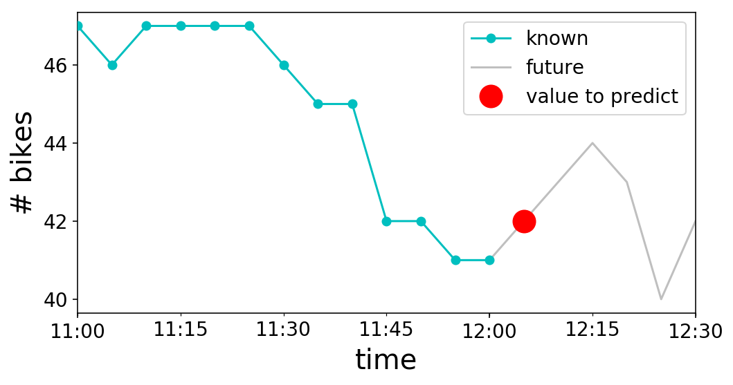
Wonderful, we’ve our time sequence. What now? Let’s take into consideration what we really need to do with it. To maintain issues easy, let’s say that we would like to have the ability to predict the subsequent worth within the time sequence. For instance, if it was midday (i.e. 12:00 PM) on Might 2nd, we’d be attempting to foretell the variety of bikes obtainable at 12:05 PM, since our time sequence is in intervals of 5 minutes. Visually, this seems to be like the next:
recognized = y.loc['2017-05-02 11:00:00':'2017-05-02 12:00:00']
unknown = y.loc['2017-05-02 12:00:00':'2017-05-02 12:30:00']
to_predict = y.loc['2017-05-02 12:05:00':'2017-05-02 12:06:00']

fig, ax = plt.subplots();
recognized.plot(ax=ax, c='c', marker='o', zorder=3);
unknown.plot(ax=ax, c='gray', alpha=0.5);
to_predict.plot(ax=ax, c='r', marker='o', markersize=16,
                linestyle='');

ax.legend(['known', 'future', 'value to predict']);
ax.set_ylabel('# bikes');
Now that we’ve framed our drawback when it comes to what we know and what we need to predict, we stroll again from whence we got here in the direction of ol’ machine studying. In time sequence, as an alternative of making a bunch of options to enter into our mannequin, we as an alternative use the historic, recognized values of our time sequence as “options” to enter right into a mannequin. The long run worth of the time sequence that we need to predict is then our goal label. Mathematically, we are going to consider $textbf{X}$ as our “characteristic matrix” or “design matrix” from machine studying. We wish to approximate $y$ with $hat{y}$, and we’ll study a operate $hat{y} = f(textbf{X})$ with a view to do that. Our $textbf{X}$ matrix consists of earlier values of $y$, our time sequence. Thus, sooner or later in time $t$,
$$mathbf{X}_{t} = mathbf{y}_{t^{prime}lt t}$$
the place I’ve considerably abused notation through the next
$$mathbf{y}_{t^{prime}lt t} equiv huge(y_{1}, y_{2}, ldots, y_{t-2}, y_{t-1} huge)$$
the place the portion on the correct denotes a vector. Consequently, if we need to predict $y$ at time $t$, then it will likely be
$$hat{y}_{t} = f(mathbf{X}_{t})$$
$$hat{y}_{t} = f(mathbf{y}_{t^{prime}lt t-1})$$
Be aware that we can not use future values to additionally predict the long run. That is why we’ve to make use of the $t-1$ worth of $textbf{X}$ to foretell $y_{t}$. In our graph from above, $t$ is 12:05 PM, the time that we try to foretell. $textbf{X}_{t-1}$ is the “recognized” cyan curve, and $y_{t}$ is the “worth to foretell” pink marker.
Now that we’re ready to think about time sequence within the snug type of $hat{y} = f(mathbf{X})$, how can we construct up the total design matrix $textbf{X}$? We wish to consider issues within the scikit-learn paradigm, the place we need to match a design matrix $textbf{X}$ by which every column is a characteristic dimension and every row is a separate “pattern” or “knowledge level”. In our case, every column of $textbf{X}$ will map to a earlier worth of $y$. We then have to think about how one can construct a number of samples.
Earlier than we construct samples, although, let’s introduce the idea of a window. Recall that $mathbf{X}_{t} = mathbf{y}_{t^{prime}lt t}$. We may use all values of $y$ up till time $t$, however this is able to rapidly get unwieldy for giant time sequence. As an alternative, we will think about some finite variety of $y$ values previous $t$. This finite vary is our window. For a window dimension $w$, $mathbf{X}_{t} = huge(y_{t-w}, y_{t-w+1},ldots, y_{t-2}, y_{t-1} huge)$.
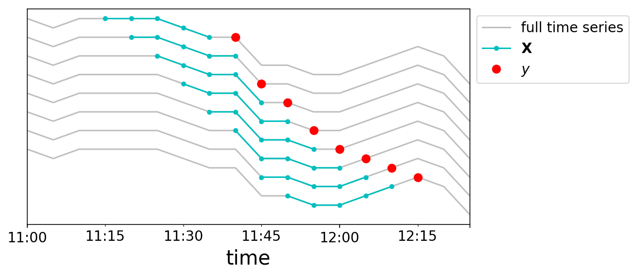
We will now construct up our knowledge samples. We are going to chop our time sequence right into a bunch of samples the place every $mathbf{X}_{t}$ is a size $w$ vector, and our targets are $y_{t}$. We’ll once more do that graphically. We take a window dimension of 5, and create 8 knowledge factors close to midday on Might 2nd. Every line plotted corresponds to a special row in our $mathbf{X}$ matrix, and the strains are vertically offset for readability.
fig, ax = plt.subplots();

begin = np.the place(y.index == '2017-05-02 11:00:00')[0][0]
center = np.the place(y.index == '2017-05-02 12:15:00')[0][0]
finish = np.the place(y.index == '2017-05-02 12:30:00')[0][0]

window = 5

for i in vary(8):

    full = y.iloc[start:end]
    prepare = y.iloc[middle - i - window:middle - i ]
    predict = y.iloc[middle - i:middle - i + 1]

    (full + 2*i).plot(ax=ax, c='gray', alpha=0.5);
    (prepare + 2*i).plot(ax=ax, c='c', markersize=4,
                       marker='o')
    (predict + 2*i).plot(ax=ax, c='r', markersize=8,
                         marker='o', linestyle='')


ax.get_yaxis().set_ticks([]);
ax.legend(['full time series',
           '$mathbf{X}$',
           '$y$'],
          bbox_to_anchor=(1, 1));
We at the moment are able to increase a dataset in an identical format to how we conventionally take into consideration machine studying issues. Let’s say that we provide you with some easy, linear mannequin. We wish to study some “characteristic weights” $mathbf{a}$, such that
$$mathbf{X}mathbf{a} = hat{mathbf{y}}$$
Recall the form of $mathbf{X}$. We’ve a row for every knowledge pattern that we’ve created. For a time sequence of size $t$, and a window dimension of $w$, then we can have $t – w$ rows. The variety of columns in $textbf{X}$ is $w$. Consequently, $textbf{a}$ shall be a length-$w$ column vector. Placing all of it collectively in matrix kind seems to be like
$$
start{bmatrix}
y_{0} & y_{1} & y_{2} & dots & y_{w – 1} cr
y_{1} & y_{2} & y_{3} & dots & y_{w} cr
vdots & vdots & vdots & ddots & vdots cr
y_{t – 2 – w} & y_{t – 1 – w} & y_{t – w} & dots & y_{t – 2} cr
y_{t – 1 – w} & y_{t – w} & y_{t – w + 1} & dots & y_{t – 1} cr
finish{bmatrix} start{bmatrix}
a_{0} cr
a_{1} cr
vdots cr
a_{w-2} cr
a_{w-1}
finish{bmatrix} = start{bmatrix}
hat{y}_{w} cr
hat{y}_{w + 1} cr
vdots cr
hat{y}_{t – 1} cr
hat{y}_{t}
finish{bmatrix}$$
How may we study these characteristic weights $textbf{a}$? Extraordinary Linear Regression shall just do high quality. Because of this our loss operate seems to be like
$$frac{1}{t-w}sumlimits_{i=w}^{i=t}huge(y_{i} – hat{y}_{i}huge)^{2}$$
We’re then free to attenuate nevertheless we would like. We’ll use scikit-learn for comfort:
#Construct our matrices

window = 5
num_samples = 8
X_mat = []
y_mat = []
for i in vary(num_samples):
    # Slice a window of options
    X_mat.append(y.iloc[middle - i - window:middle - i].values)
    y_mat.append(y.iloc[middle - i:middle - i + 1].values)

X_mat = np.vstack(X_mat)
y_mat = np.concatenate(y_mat)

assert X_mat.form == (num_samples, window)
assert len(y_mat) == num_samples
from sklearn.linear_model import LinearRegression
from sklearn.metrics import r2_score

lr = LinearRegression(fit_intercept=False)
lr = lr.match(X_mat, y_mat)
y_pred = lr.predict(X_mat)
fig, ax = plt.subplots(figsize=(6, 6));

ax.scatter(y_pred, y_mat);

one_to_one = np.arange(y_mat.min()-2, y_mat.max()+2)
ax.plot(one_to_one, one_to_one, c='r', linestyle='--');

ax.set_xlim((one_to_one[0], one_to_one[-1]));
ax.set_ylim((one_to_one[0], one_to_one[-1]));
ax.set_xlabel('Predicted');
ax.set_ylabel('True');
ax.set_title(f'$R^{2}$ = {r2_score(y_mat, y_pred):3.2f}');
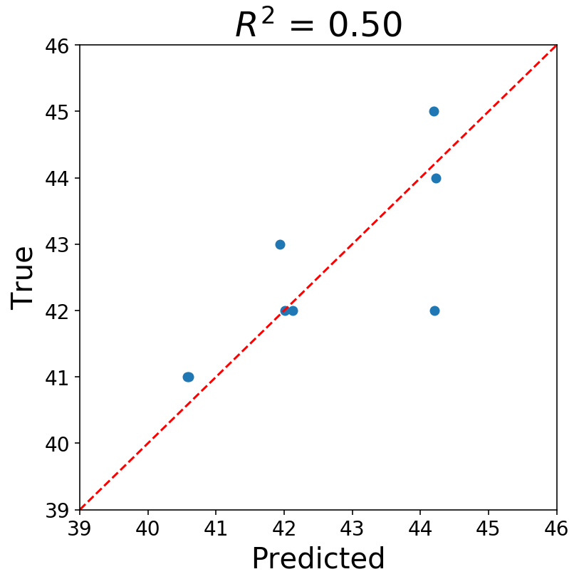
Now you’ll be able to ask your self if what we’ve performed is okay, and the reply ought to most likely be “No”. I’m assuming most statisticians could be extraordinarily uncomfortable proper now. There’s all types of points, however, at the beginning, our knowledge factors are most assuredly not IID. A lot of the statistical points with the above roll up into the idea that the information have to be stationary earlier than working a regression. Additionally, our time sequence consists of strictly integer values, and utilizing steady fashions appears suspect to me.
Nonetheless, I’m high quality with what we did. The purpose of the above was to point out that it’s potential to forged a time sequence drawback into a well-recognized format.
By the way in which, what we’ve performed is outlined and solved an autoregressive mannequin which is the primary two letters within the notorious ARIMA household of fashions.
Now that we’ve seen how one can flip a time sequence drawback right into a typical supervised studying drawback, one can simply add options to the mannequin as additional columns within the design matrix, $mathbf{X}$. The difficult half about time sequence is that, since you’re predicting the long run, you could know what the long run values of your options shall be. For instance, we may add in a binary characteristic indicating whether or not or not there may be rain into our bike availablility forecaster. Whereas this might probably be helpful for growing accuracy on the coaching knowledge, we would wish to have the ability to precisely forecast the climate with a view to forecast the time sequence far into the long run, and everyone knows how onerous climate forecasting is! Normally, constructing coaching and take a look at knowledge for options that change with time is troublesome, as it may be straightforward to leak data from the long run into the previous.
Lastly, I’d additionally wish to level out that, whereas we selected to make use of Linear Regression as our mannequin, we may have used every other sort of mannequin, similar to a random forest or neural community.
Within the subsequent submit, I’ll stroll by means of how we will appropriately construct up a design matrix, and we’ll tackle the duty of forecasting bike availability.
