Final put up I described how I collected implicit suggestions knowledge from the web site Sketchfab. I then claimed I might write about the best way to truly construct a suggestion system with this knowledge. Properly, right here we’re! Let’s construct.
I feel the very best place to begin when trying into implicit suggestions recommenders is with the mannequin outlined within the traditional paper “Collaborative Filtering for Implicit Suggestions Datasets” by Koren et.al. (warning: pdf hyperlink). I’ve seen many names within the literature and machine studying libraries for this mannequin. I’ll name it Weighted Regularized Matrix Factorization (WRMF) which tends to be a reputation used pretty usually. WRMF is just like the traditional rock of implicit matrix factorization. It might not be the trendiest, however it is going to by no means exit of fashion. And, everytime I exploit it, I do know that I’m assured to love what I get out. Particularly, this mannequin makes cheap intuitive sense, it’s scalable, and, most significantly, I’ve discovered it simple to tune. There are a lot fewer hyperparameters than, say, stochastic gradient descent fashions.
When you recall from my put up on Express Suggestions Matrix Factorization, we had a loss operate (with out biases) that regarded like:
$$L_{exp} = sumlimits_{u,i in S}(r_{ui} – textbf{x}_{u}^{intercal} cdot{} textbf{y}_{i})^{2} + lambda_{x} sumlimits_{u} leftVert textbf{x}_{u} rightVert^{2} + lambda_{y} sumlimits_{u} leftVert textbf{y}_{i} rightVert^{2}$$
the place $r_{ui}$ is a component of the matrix of user-item rankings, $textbf{x}_{u}$ ($textbf{y}_{i}$) are person $u$’s (merchandise $i$’s) latent components, and $S$ was the set of all user-item rankings. WRMF is solely a modification of this loss operate:
$$L_{WRMF} = sumlimits_{u,i}c_{ui} large( p_{ui} – textbf{x}_{u}^{intercal} cdot{} textbf{y}_{i} large) ^{2} + lambda_{x} sumlimits_{u} leftVert textbf{x}_{u} rightVert^{2} + lambda_{y} sumlimits_{u} leftVert textbf{y}_{i} rightVert^{2}$$
Right here, we aren’t summing of over parts of $S$ however as a substitute over our total matrix. Recall that with implicit suggestions, we wouldn’t have rankings anymore; quite, we now have customers’ preferences for gadgets. Within the WRMF loss operate, the rankings matrix $r_{ui}$ has been changed with a desire matrix $p_{ui}$. We make the idea that if a person has interacted in any respect with an merchandise, then $p_{ui} = 1$. In any other case, $p_{ui} = 0$.
The opposite new time period within the loss operate is $c_{ui}$. We name this the boldness matrix, and it roughly describes how assured we’re that person $u$ does in truth have desire $p_{ui}$ for merchandise $i$. Within the paper, one of many confidence formulation that the authors think about is linear within the variety of interactions. If we take $d_{ui}$ to be the variety of instances a person has clicked on an merchandise on an internet site, then
$$c_{ui} = 1 + alpha d_{ui}$$
the place $alpha$ is a few hyperparameter decided by cross validation. Within the case of the Sketchfab knowledge, we solely have binary “likes”, so $d_{ui} in {0, 1}$
To take a step again, WRMF doesn’t make the idea {that a} person who has not interacted with an merchandise doesn’t like the merchandise. WRMF does assume that that person has a damaging desire in the direction of that merchandise, however we are able to select how assured we’re in that assumption by means of the boldness hyperparameter.
Now, I might undergo the entire derivation in gory latex of the best way to optimize this algorithm á la my earlier express MF put up, however different individuals have already accomplished this many instances over. Right here’s an excellent StackOverflow reply, or, should you like your derivations in Dirac notation, then checkout Sudeep Das’ put up.
WRMF Libraries
There are a selection of locations to seek out open supply code which implements WRMF. The most well-liked methodology of optimizing the loss operate is thru Alternating Least Squares. This tends be much less difficult to tune than stochastic gradient descent, and the mannequin is embarrassingly parallel.
The primary code I noticed for this algorithm was from Chris Johnson’s repo. This code is in python, properly makes use of sparse matrices, and usually will get the job accomplished. Thierry Bertin-Mahieux then took this code and parallelized it utilizing the python multiprocessing library. This offers an honest speedup with no loss in accuracy.
The individuals at Quora got here out with a library referred to as qmf which is parellized and written in C++. I haven’t used it, however it’s presumably sooner than the multiprocessing python model. Lastly, Ben Frederickson went and wrote parallelized code in pure Cython right here. This blows the opposite python variations out of the water when it comes to efficiency and is one way or the other sooner than qmf (which appears odd).
Anywho, I ended up utilizing Ben’s library for this put up as a result of (1) I might keep in python, and (2) it’s tremendous quick. I forked the library and wrote a small class to wrap the algorithm to make it simple to run grid searches and calculate studying curves. Be at liberty to take a look at my fork right here, although I didn’t write any exams so use at your personal danger 🙂
Massaging the info
Now that that’s out of the way in which, let’s practice a WRMF mannequin so we are able to lastly suggest some Sketchfab fashions!
Step one is to load the info and rework it into an interactions matrix of measurement “variety of customers” by “variety of gadgets”. The info is presently saved as a csv with every row denoting a mannequin {that a} person has “appreciated” on the Sketchfab web site. The primary column is the identify of the mannequin, the second column is the distinctive mannequin ID (mid), and the third column is the anonymized person ID (uid).
%matplotlib inline
import matplotlib.pyplot as plt
import pandas as pd
import numpy as np
import scipy.sparse as sparse
import pickle
import csv
import implicit
import itertools
import copy
plt.type.use('ggplot')
df = pd.read_csv('../knowledge/model_likes_anon.psv',
                 sep='|', quoting=csv.QUOTE_MINIMAL,
                 quotechar='')
df.head()
| modelname | mid | uid | |
|---|---|---|---|
| 0 | 3D fanart Noel From Sora no Methodology | 5dcebcfaedbd4e7b8a27bd1ae55f1ac3 | 7ac1b40648fff523d7220a5d07b04d9b |
| 1 | 3D fanart Noel From Sora no Methodology | 5dcebcfaedbd4e7b8a27bd1ae55f1ac3 | 2b4ad286afe3369d39f1bb7aa2528bc7 |
| 2 | 3D fanart Noel From Sora no Methodology | 5dcebcfaedbd4e7b8a27bd1ae55f1ac3 | 1bf0993ebab175a896ac8003bed91b4b |
| 3 | 3D fanart Noel From Sora no Methodology | 5dcebcfaedbd4e7b8a27bd1ae55f1ac3 | 6484211de8b9a023a7d9ab1641d22e7c |
| 4 | 3D fanart Noel From Sora no Methodology | 5dcebcfaedbd4e7b8a27bd1ae55f1ac3 | 1109ee298494fbd192e27878432c718a |
print('Duplicated rows: ' + str(df.duplicated().sum()))
print('That's bizarre - let's simply drop them')
df.drop_duplicates(inplace=True)
Duplicated rows 155
That is bizarre - let's simply drop them
df = df[['uid', 'mid']]
df.head()
| uid | mid | |
|---|---|---|
| 0 | 7ac1b40648fff523d7220a5d07b04d9b | 5dcebcfaedbd4e7b8a27bd1ae55f1ac3 |
| 1 | 2b4ad286afe3369d39f1bb7aa2528bc7 | 5dcebcfaedbd4e7b8a27bd1ae55f1ac3 |
| 2 | 1bf0993ebab175a896ac8003bed91b4b | 5dcebcfaedbd4e7b8a27bd1ae55f1ac3 |
| 3 | 6484211de8b9a023a7d9ab1641d22e7c | 5dcebcfaedbd4e7b8a27bd1ae55f1ac3 |
| 4 | 1109ee298494fbd192e27878432c718a | 5dcebcfaedbd4e7b8a27bd1ae55f1ac3 |
n_users = df.uid.distinctive().form[0]
n_items = df.mid.distinctive().form[0]

print('Variety of customers: {}'.format(n_users))
print('Variety of fashions: {}'.format(n_items))
print('Sparsity: {:4.3f}%'.format(float(df.form[0]) / float(n_users*n_items) * 100))
Variety of customers: 62583
Variety of fashions: 28806
Sparsity: 0.035%
Whereas implicit suggestions excel the place knowledge is sparse, it will possibly usually be useful to make the interactions matrix just a little extra dense. We restricted our knowledge assortment to fashions that had at the very least 5 likes. Nonetheless, it might not be the case that each person has appreciated at the very least 5 fashions. Let’s go forward and knock out customers that loved fewer than 5 fashions. This might presumably imply that some fashions find yourself with fewer than 5 likes as soon as these customers are knocked out, so we should alternate forwards and backwards knocking customers and fashions out till issues stabilize.
def threshold_likes(df, uid_min, mid_min):
    n_users = df.uid.distinctive().form[0]
    n_items = df.mid.distinctive().form[0]
    sparsity = float(df.form[0]) / float(n_users*n_items) * 100
    print('Beginning likes information')
    print('Variety of customers: {}'.format(n_users))
    print('Variety of fashions: {}'.format(n_items))
    print('Sparsity: {:4.3f}%'.format(sparsity))

    accomplished = False
    whereas not accomplished:
        starting_shape = df.form[0]
        mid_counts = df.groupby('uid').mid.rely()
        df = df[~df.uid.isin(mid_counts[mid_counts < mid_min].index.tolist())]
        uid_counts = df.groupby('mid').uid.rely()
        df = df[~df.mid.isin(uid_counts[uid_counts < uid_min].index.tolist())]
        ending_shape = df.form[0]
        if starting_shape == ending_shape:
            accomplished = True

    assert(df.groupby('uid').mid.rely().min() >= mid_min)
    assert(df.groupby('mid').uid.rely().min() >= uid_min)

    n_users = df.uid.distinctive().form[0]
    n_items = df.mid.distinctive().form[0]
    sparsity = float(df.form[0]) / float(n_users*n_items) * 100
    print('Ending likes information')
    print('Variety of customers: {}'.format(n_users))
    print('Variety of fashions: {}'.format(n_items))
    print('Sparsity: {:4.3f}%'.format(sparsity))
    return df
df_lim = threshold_likes(df, 5, 5)
Beginning likes information
Variety of customers: 62583
Variety of fashions: 28806
Sparsity: 0.035%
Ending likes information
Variety of customers: 15274
Variety of fashions: 25655
Sparsity: 0.140%
Good, we’re above 0.1% which ought to be appropriate for making first rate suggestions. We now have to map every uid and mid to a row and column, respectively, for our interactions, or “likes” matrix. This may be accomplished merely with Python dictionaries
# Create mappings
mid_to_idx = {}
idx_to_mid = {}
for (idx, mid) in enumerate(df_lim.mid.distinctive().tolist()):
    mid_to_idx[mid] = idx
    idx_to_mid[idx] = mid

uid_to_idx = {}
idx_to_uid = {}
for (idx, uid) in enumerate(df_lim.uid.distinctive().tolist()):
    uid_to_idx[uid] = idx
    idx_to_uid[idx] = uid
The final step is to truly construct the matrix. We are going to use sparse matrices in order to not take up an excessive amount of reminiscence. Sparse matrices are difficult as a result of they arrive in lots of types, and there are large efficiency tradeoffs between them. Beneath is a brilliant gradual strategy to construct a likes matrix. I attempted working %%timeit however obtained bored ready for it to complete.
# # Do not do that!
# num_users = df_lim.uid.distinctive().form[0]
# num_items = df_lim.mid.distinctive().form[0]
# likes = sparse.csr_matrix((num_users, num_items), dtype=np.float64)
# for row in df_lim.itertuples():
#     likes[uid_to_idx[uid], mid_to_idx[row.mid]] = 1.0
Alternatively, the under is fairly rattling quick contemplating we’re constructing a matrix of half 1,000,000 likes.
def map_ids(row, mapper):
    return mapper[row]
%%timeit
I = df_lim.uid.apply(map_ids, args=[uid_to_idx]).as_matrix()
J = df_lim.mid.apply(map_ids, args=[mid_to_idx]).as_matrix()
V = np.ones(I.form[0])
likes = sparse.coo_matrix((V, (I, J)), dtype=np.float64)
likes = likes.tocsr()
1 loop, finest of three: 876 ms per loop
I = df_lim.uid.apply(map_ids, args=[uid_to_idx]).as_matrix()
J = df_lim.mid.apply(map_ids, args=[mid_to_idx]).as_matrix()
V = np.ones(I.form[0])
likes = sparse.coo_matrix((V, (I, J)), dtype=np.float64)
likes = likes.tocsr()
Cross-validation: Splitsville
Okay, we obtained a likes matrix and want to separate it into coaching and check matrices. I do that a bit trickily (which is perhaps a phrase?). I want to observe precision@okay as my optimization metric later. A okay of 5 could be good. Nonetheless, if I transfer 5 gadgets from coaching to check for a number of the customers, then they might not have any knowledge left within the coaching set (keep in mind that they had a minimal 5 likes). Thus, the train_test_split solely appears to be like for individuals who have at the very least 2*okay (10 on this case) likes earlier than shifting a few of their knowledge to the check set. This clearly biases our cross-validation in the direction of customers with extra likes. So it goes.
def train_test_split(rankings, split_count, fraction=None):
    """
    Cut up suggestion knowledge into practice and check units

    Params
    ------
    rankings : scipy.sparse matrix
        Interactions between customers and gadgets.
    split_count : int
        Variety of user-item-interactions per person to maneuver
        from coaching to check set.
    fractions : float
        Fraction of customers to separate off a few of their
        interactions into check set. If None, then all
        customers are thought-about.
    """
    # Be aware: probably not the quickest strategy to do issues under.
    practice = rankings.copy().tocoo()
    check = sparse.lil_matrix(practice.form)

    if fraction:
        strive:
            user_index = np.random.selection(
                np.the place(np.bincount(practice.row) >= split_count * 2)[0],
                change=False,
                measurement=np.int32(np.ground(fraction * practice.form[0]))
            ).tolist()
        besides:
            print(('Not sufficient customers with > {} '
                  'interactions for fraction of {}')
                  .format(2*okay, fraction))
            increase
    else:
        user_index = vary(practice.form[0])

    practice = practice.tolil()

    for person in user_index:
        test_ratings = np.random.selection(rankings.getrow(person).indices,
                                        measurement=split_count,
                                        change=False)
        practice[user, test_ratings] = 0.
        # These are simply 1.0 proper now
        check[user, test_ratings] = rankings[user, test_ratings]


    # Check and coaching are actually disjoint
    assert(practice.multiply(check).nnz == 0)
    return practice.tocsr(), check.tocsr(), user_index
practice, check, user_index = train_test_split(likes, 5, fraction=0.2)
Cross-validation: Grid search
Now that the info is cut up into coaching and check matrices, let’s run an enormous grid search to optimize our hyperparameters. We’ve 4 parameters that we want to optimize:
num_factors: The variety of latent components, or diploma of dimensionality in our mannequin.regularization: Scale of regularization for each person and merchandise components.alpha: Our confidence scaling time period.iterations: Variety of iterations to run Alternating Least Squares optimization.
I’m going to trace imply squared error (MSE) and precision at okay (p@okay), however I primarily care in regards to the later. I’ve written some features under to assist with metric calculations and making the coaching log printout look good. I’m going to calculate a bunch of studying curves (that’s, consider efficiency metrics at varied phases of the coaching course of) for a bunch of various hyperparameter combos. Props to scikit-learn for being open supply and letting me mainly crib their GridSearchCV code.
from sklearn.metrics import mean_squared_error
def calculate_mse(mannequin, rankings, user_index=None):
    preds = mannequin.predict_for_customers()
    if user_index:
        return mean_squared_error(rankings[user_index, :].toarray().ravel(),
                                  preds[user_index, :].ravel())

    return mean_squared_error(rankings.toarray().ravel(),
                              preds.ravel())
def precision_at_k(mannequin, rankings, okay=5, user_index=None):
    if not user_index:
        user_index = vary(rankings.form[0])
    rankings = rankings.tocsr()
    precisions = []
    # Be aware: line under might grow to be infeasible for big datasets.
    predictions = mannequin.predict_for_customers()
    for person in user_index:
        # In case of enormous dataset, compute predictions row-by-row like under
        # predictions = np.array([model.predict(row, i) for i in xrange(ratings.shape[1])])
        top_k = np.argsort(-predictions[user, :])[:k]
        labels = rankings.getrow(person).indices
        precision = float(len(set(top_k) & set(labels))) / float(okay)
        precisions.append(precision)
    return np.imply(precisions)
def print_log(row, header=False, spacing=12):
    prime = ''
    center = ''
    backside = ''
    for r in row:
        prime += '+{}'.format('-'*spacing)
        if isinstance(r, str):
            center += '| {0:^{1}} '.format(r, spacing-2)
        elif isinstance(r, int):
            center += '| {0:^{1}} '.format(r, spacing-2)
        elif isinstance(r, float):
            center += '| {0:^{1}.5f} '.format(r, spacing-2)
        backside += '+{}'.format('='*spacing)
    prime += '+'
    center += '|'
    backside += '+'
    if header:
        print(prime)
        print(center)
        print(backside)
    else:
        print(center)
        print(prime)
def learning_curve(mannequin, practice, check, epochs, okay=5, user_index=None):
    if not user_index:
        user_index = vary(practice.form[0])
    prev_epoch = 0
    train_precision = []
    train_mse = []
    test_precision = []
    test_mse = []

    headers = ['epochs', 'p@k train', 'p@k test',
               'mse train', 'mse test']
    print_log(headers, header=True)

    for epoch in epochs:
        mannequin.iterations = epoch - prev_epoch
        if not hasattr(mannequin, 'user_vectors'):
            mannequin.match(practice)
        else:
            mannequin.fit_partial(practice)
        train_mse.append(calculate_mse(mannequin, practice, user_index))
        train_precision.append(precision_at_k(mannequin, practice, okay, user_index))
        test_mse.append(calculate_mse(mannequin, check, user_index))
        test_precision.append(precision_at_k(mannequin, check, okay, user_index))
        row = [epoch, train_precision[-1], test_precision[-1],
               train_mse[-1], test_mse[-1]]
        print_log(row)
        prev_epoch = epoch
    return mannequin, train_precision, train_mse, test_precision, test_mse
def grid_search_learning_curve(base_model, practice, check, param_grid,
                               user_index=None, patk=5, epochs=vary(2, 40, 2)):
    """
    "Impressed" (stolen) from sklearn gridsearch
    https://github.com/scikit-learn/scikit-learn/blob/grasp/sklearn/model_selection/_search.py
    """
    curves = []
    keys, values = zip(*param_grid.gadgets())
    for v in itertools.product(*values):
        params = dict(zip(keys, v))
        this_model = copy.deepcopy(base_model)
        print_line = []
        for okay, v in params.gadgets():
            setattr(this_model, okay, v)
            print_line.append((okay, v))

        print(' | '.be a part of('{}: {}'.format(okay, v) for (okay, v) in print_line))
        _, train_patk, train_mse, test_patk, test_mse = learning_curve(this_model, practice, check,
                                                                epochs, okay=patk, user_index=user_index)
        curves.append({'params': params,
                       'patk': {'practice': train_patk, 'check': test_patk},
                       'mse': {'practice': train_mse, 'check': test_mse}})
    return curves
Please notice that the under parameter grid is fucking enormous and took like 2 days to run on my 6-year outdated 4-core i5. It seems that the efficiency metrics features are literally a great bit slower than the coaching course of. These features could possibly be merely paralellized – one thing for me to do on a later date.
param_grid = {'num_factors': [10, 20, 40, 80, 120],
              'regularization': [0.0, 1e-5, 1e-3, 1e-1, 1e1, 1e2],
              'alpha': [1, 10, 50, 100, 500, 1000]}
base_model = implicit.ALS()
curves = grid_search_learning_curve(base_model, practice, check,
                                    param_grid,
                                    user_index=user_index,
                                    patk=5)
The coaching log is ridculously lengthy, however be at liberty to click on right here and test it out. In any other case, right here’s the printout of the very best run:
alpha: 50 | num_factors: 40 | regularization: 0.1
+------------+------------+------------+------------+------------+
|   epochs   | p@okay practice  |  p@okay check  | mse practice  |  mse check  |
+============+============+============+============+============+
|     2      |  0.33988   |  0.02541   |  0.01333   |  0.01403   |
+------------+------------+------------+------------+------------+
|     4      |  0.31395   |  0.03916   |  0.01296   |  0.01377   |
+------------+------------+------------+------------+------------+
|     6      |  0.30085   |  0.04231   |  0.01288   |  0.01372   |
+------------+------------+------------+------------+------------+
|     8      |  0.29175   |  0.04231   |  0.01285   |  0.01370   |
+------------+------------+------------+------------+------------+
|     10     |  0.28638   |  0.04407   |  0.01284   |  0.01370   |
+------------+------------+------------+------------+------------+
|     12     |  0.28684   |  0.04492   |  0.01284   |  0.01371   |
+------------+------------+------------+------------+------------+
|     14     |  0.28533   |  0.04571   |  0.01285   |  0.01371   |
+------------+------------+------------+------------+------------+
|     16     |  0.28389   |  0.04689   |  0.01285   |  0.01372   |
+------------+------------+------------+------------+------------+
|     18     |  0.28454   |  0.04695   |  0.01286   |  0.01373   |
+------------+------------+------------+------------+------------+
|     20     |  0.28454   |  0.04728   |  0.01287   |  0.01374   |
+------------+------------+------------+------------+------------+
|     22     |  0.28409   |  0.04761   |  0.01288   |  0.01376   |
+------------+------------+------------+------------+------------+
|     24     |  0.28251   |  0.04689   |  0.01289   |  0.01377   |
+------------+------------+------------+------------+------------+
|     26     |  0.28186   |  0.04656   |  0.01290   |  0.01378   |
+------------+------------+------------+------------+------------+
|     28     |  0.28199   |  0.04676   |  0.01291   |  0.01379   |
+------------+------------+------------+------------+------------+
|     30     |  0.28127   |  0.04669   |  0.01292   |  0.01380   |
+------------+------------+------------+------------+------------+
|     32     |  0.28173   |  0.04650   |  0.01292   |  0.01381   |
+------------+------------+------------+------------+------------+
|     34     |  0.28153   |  0.04650   |  0.01293   |  0.01382   |
+------------+------------+------------+------------+------------+
|     36     |  0.28166   |  0.04604   |  0.01294   |  0.01382   |
+------------+------------+------------+------------+------------+
|     38     |  0.28153   |  0.04637   |  0.01295   |  0.01383   |
+------------+------------+------------+------------+------------+
Let’s see what the educational curve appears to be like like for our greatest run.
best_curves = sorted(curves, key=lambda x: max(x['patk']['test']), reverse=True)
print(best_curves[0]['params'])
max_score = max(best_curves[0]['patk']['test'])
print(max_score)
iterations = vary(2, 40, 2)[best_curves[0]['patk']['test'].index(max_score)]
print('Epoch: {}'.format(iterations))
{'alpha': 50, 'num_factors': 40, 'regularization': 0.1}
0.0476096922069
Epoch: 22
import seaborn as sns
sns.set_style('white')
fig, ax = plt.subplots()
sns.despine(fig);
plt.plot(epochs, best_curves[0]['patk']['test']);
plt.xlabel('Epochs', fontsize=24);
plt.ylabel('Check p@okay', fontsize=24);
plt.xticks(fontsize=18);
plt.yticks(fontsize=18);
plt.title('Finest studying curve', fontsize=30);
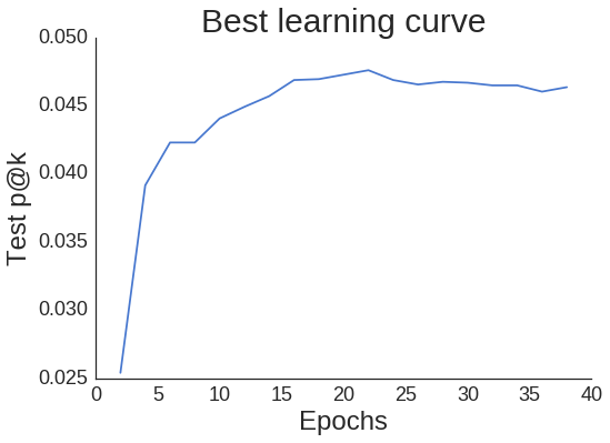
Whereas the curve is a bit jagged, it doesn’t lower too considerably as we transfer previous our greatest epoch of twenty-two. This implies we wouldn’t have to be tremendous cautious implementing early stopping (if we take p@okay to be the one metric that we care about).
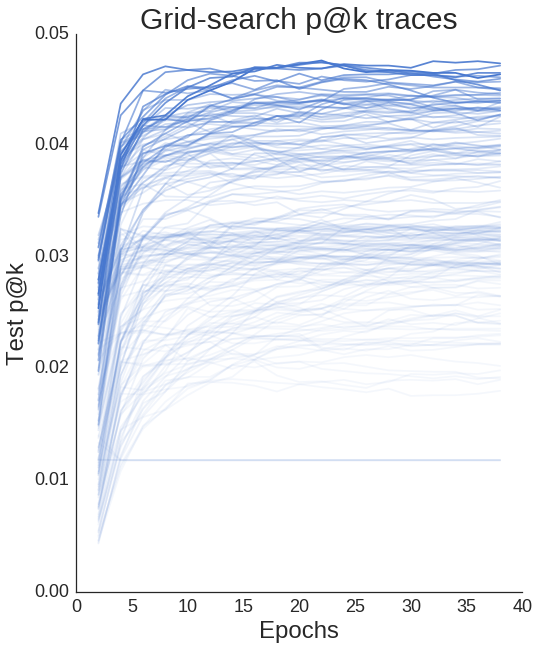
We are able to plot all of our studying curves and see that variations in hyperparameters positively make a distinction in efficiency.
all_test_patks = [x['patk']['test'] for x in best_curves]
fig, ax = plt.subplots(figsize=(8, 10));
sns.despine(fig);
epochs = vary(2, 40, 2)
totes = len(all_test_patks)
for i, test_patk in enumerate(all_test_patks):
    ax.plot(epochs, test_patk,
             alpha=1/(.1*i+1),
             c=sns.color_palette()[0]);

plt.xlabel('Epochs', fontsize=24);
plt.ylabel('Check p@okay', fontsize=24);
plt.xticks(fontsize=18);
plt.yticks(fontsize=18);
plt.title('Grid-search p@okay traces', fontsize=30);
Rec-a-sketch
In spite of everything that, we lastly have some optimum hyperparameters. We might now do a finer grid search or have a look at how various the ratio between person and merchandise regularization results outcomes, however I don’t really feel like ready one other 2 days…
We’ll now practice a WRMF mannequin on all of our knowledge with the optimum hyper parameters and visualize some item-to-item suggestions. Consumer-to-item suggestions are a bit harder to visualise and get a really feel for a way correct they might be.
params = best_curves[0]['params']
params['iterations'] = vary(2, 40, 2)[best_curves[0]['patk']['test'].index(max_score)]
bestALS = implicit.ALS(**params)
To get item-to-item suggestions, I made a small methodology predict_for_items within the ALS class. That is basically only a dot product between each mixture of merchandise vectors. When you let norm=True (the default), then this dot product is normalized by the norm of every merchandise vector ensuing within the cosine similarity. This tells us how comparable two gadgets are within the embedded, or latent area.
    def predict_for_items(self, norm=True):
        """Advocate merchandise for all merchandise"""
        pred = self.item_vectors.dot(self.item_vectors.T)
        if norm:
            norms = np.array([np.sqrt(np.diagonal(pred))])
            pred = pred / norms / norms.T
        return pred
item_similarities = bestALS.predict_for_items()
Let’s now visualize a number of the fashions and their related suggestions to get a really feel for a way effectively our recommender is working. We are able to merely question the sketchfab api to seize the fashions’ thumbnails. Beneath is a helper operate, that makes use of the merchandise similarities, an index, and the index-to-mid mapper to return a listing of the suggestions’ thumbnail urls. Be aware that the primary suggestion is all the time the mannequin itself because of it having a cosine similarity of 1 with itself.
import requests
def get_thumbnails(sim, idx, idx_to_mid, N=10):
    row = sim[idx, :]
    thumbs = []
    for x in np.argsort(-row)[:N]:
        response = requests.get('https://sketchfab.com/i/fashions/{}'.format(idx_to_mid[x])).json()
        thumb = [x['url'] for x in response['thumbnails']['images'] if x['width'] == 200 and x['height']==200]
        if not thumb:
            print('no thumbnail')
        else:
            thumb = thumb[0]
        thumbs.append(thumb)
    return thumbs
thumbs = get_thumbnails(item_similarities, 0, idx_to_mid)
https://dg5bepmjyhz9h.cloudfront.web/urls/5dcebcfaedbd4e7b8a27bd1ae55f1ac3/dist/thumbnails/a59f9de0148e4986a181483f47826fe0/200x200.jpeg
We are able to now show the photographs utilizing some HTML and core IPython features.
from IPython.show import show, HTML

def display_thumbs(thumbs, N=5):
    thumb_html = "<img type='width: 160px; margin: 0px;
                  border: 1px strong black;' src='{}' />"
    pictures = ''
    show(HTML('<font measurement=5>'+'Enter Mannequin'+'</font>'))
    show(HTML(thumb_html.format(thumbs[0])))
    show(HTML('<font measurement=5>'+'Related Fashions'+'</font>'))

    for url in thumbs[1:N+1]:
        pictures += thumb_html.format(url)
    show(HTML(pictures))
Whereas the suggestions might not be excellent (see police automotive + inexperienced monster above), it’s apparent that our suggestion mannequin has realized similarities.
Take a step again and take into consideration this for a second:
Our algorithm is aware of nothing about what these fashions appear like, what tags they might have on them, or something in regards to the artists. The algorithm merely is aware of which customers have appreciated which fashions. Fairly creepy, huh?
What’s subsequent?
At present we realized Weighted Regularized Matrix Factorization, the traditional rock of implicit MF. Subsequent time, we’ll study one other methodology of optimizing implicit suggestions fashions referred to as Studying to Rank. With Studying to Rank fashions, we’ll be capable to embody additional details about the fashions and customers such because the classes and tags assigned to the fashions. After that, we’ll see how an unsupervised suggestion utilizing pictures and pretrained neural networks compares to those strategies, after which lastly we’ll construct a flask app to serve these suggestions to an finish person.
Keep tuned!
