
Random Forests are versatile and highly effective in relation to tabular knowledge. Do in addition they work for time-series forecasting? Let’s discover out.

Right now, Deep Studying dominates many areas of contemporary machine studying. However, Choice Tree based mostly fashions nonetheless shine significantly for tabular knowledge. If you happen to search for the profitable options of respective Kaggle challenges, likelihood is excessive {that a} tree mannequin is amongst them.
A key benefit of tree approaches is that they sometimes don’t require an excessive amount of fine-tuning for cheap outcomes. That is in stark distinction to Deep Studying. Right here, completely different topologies and architectures can lead to dramatical variations in mannequin efficiency.
For time-series forecasting, choice bushes are usually not as easy as for tabular knowledge, although:
As you most likely know, becoming any choice tree based mostly strategies requires each enter and output variables. In a univariate time-series downside, nevertheless, we normally solely have our time-series as a goal.
To work round this problem, we have to increase the time-series to grow to be appropriate for tree fashions. Allow us to talk about two intuitive, but false approaches and why they fail first. Clearly, the problems generalize to all Choice Tree ensemble strategies.
Choice Tree forecasting as regression in opposition to time
Most likely probably the most intuitive strategy is to contemplate the noticed time-series as a operate of time itself, i.e.

With some i.i.d. stochastic additive error time period. In an earlier article, I’ve already made some remarks on why regression in opposition to time itself is problematic. For tree based mostly fashions, there may be one other downside:
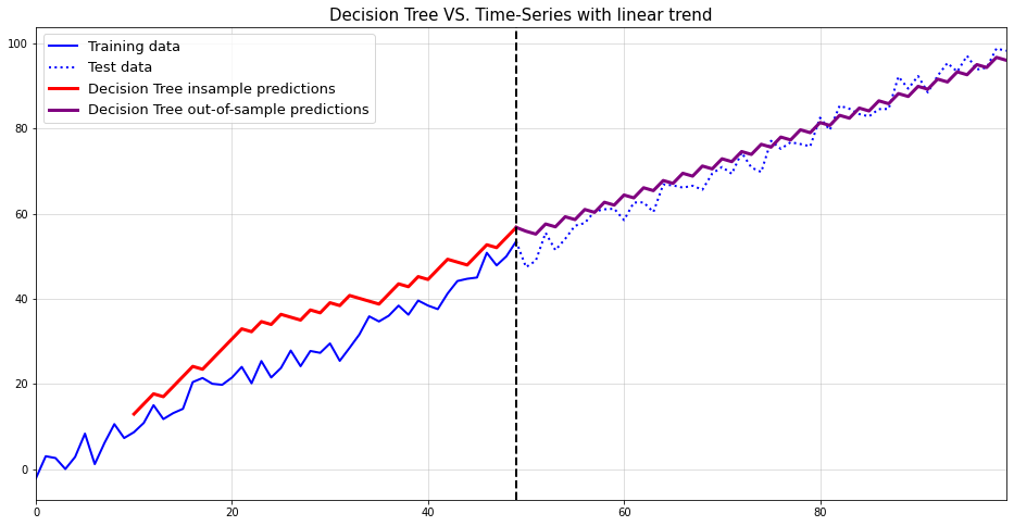
Choice Timber for regression in opposition to time can’t extrapolate into the long run.
By development, Choice Tree predictions are averages of subsets of the coaching dataset. These subsets are fashioned by splitting the area of enter knowledge into axis-parallel hyper rectangles. Then, for every hyper rectangle, we take the typical of all remark outputs inside these rectangles as a prediction.
For regression in opposition to time, these hyper rectangles are merely splits of time intervals. Extra precisely, these intervals are mutually unique and utterly exhaustive.
Predictions are then the arithmetic technique of the time-series observations inside these intervals. Mathematically, this roughly interprets to

Contemplate now utilizing this mannequin to foretell the time-series at a while sooner or later. This reduces the above system to the next:

In phrases: For any forecast, our mannequin all the time predicts the typical of the ultimate coaching interval. Which is clearly ineffective…
Allow us to visualize this problem on a fast toy instance:

The identical points clearly come up for seasonal patterns as nicely:

To generalize the above in a single sentence:
Choice Timber fail for out-of-distribution knowledge however in regression in opposition to time, each future time limit is out-of-distribution.
Thus, we have to discover a completely different strategy.
A much more promising strategy is the auto-regressive one. Right here, we merely view the way forward for a random variable as depending on its previous realizations.

Whereas this strategy is less complicated to deal with than regression on time, it doesn’t come with out a price:
- The time-series have to be noticed at equi-distant timestamps: In case your time-series is measured at random occasions, you can not use this strategy with out additional changes.
- The time-series shouldn’t comprise lacking values: For a lot of time-series fashions, this requirement just isn’t obligatory. Our Choice Tree/Random Forest forecaster, nevertheless, would require a totally noticed time-series.
As these caveats are frequent for hottest time-series approaches, they aren’t an excessive amount of of a difficulty.
Now, earlier than leaping into an instance, we have to take a one other take a look at a beforehand mentioned problem: Tree based mostly fashions can solely predict inside the vary of coaching knowledge. This suggests that we can’t simply match a Choice Tree or Random Forest to mannequin auto-regressive dependencies.
To exemplify this problem, let’s do one other instance:

Once more, not helpful in any respect. To repair this final problem, we have to first take away the pattern. Then we are able to match the mannequin, forecast the time-series and ‘re-trend’ the forecast.
For de-trending, we principally have two choices:
- Match a linear pattern mannequin — right here we regress the time-series in opposition to time in a linear regression mannequin. Its predictions are then subtracted from the coaching knowledge to create a stationary time-series. This removes a continuing, deterministic pattern.
- Use first-differences — on this strategy, we rework the time-series by way of first order differencing. Along with the deterministic pattern, this strategy also can take away stochastic tendencies.
As most time-series are pushed by randomness, the second strategy seems extra cheap. Thus, we now goal to forecast the remodeled time-series

by an autoregressive mannequin, i.e.

Clearly, differencing and lagging take away some observations from our coaching knowledge. Some care needs to be taken to not take away an excessive amount of info that means. I.e. don’t use too many lagged variables in case your dataset is small.
To acquire a forecast for the unique time-series we have to retransform the differenced forecast by way of

and, recursively for additional forward forecasts:

For our working instance this lastly results in an affordable answer:
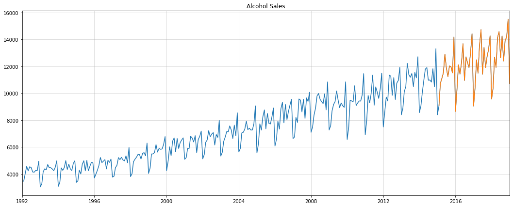
Allow us to now apply the above strategy to a real-world dataset. We use the alcohol gross sales knowledge from the St. Louis Fed database. For analysis, we use the final 4 years as a holdout set:
Since a single Choice Tree could be boring at greatest and inaccurate at worst, we’ll use a Random Forest as an alternative. Apart from the everyday efficiency enhancements, Random Forests enable us to generate forecast intervals.
To create Random Forest forecast intervals, we proceed as follows:
- Practice an autoregressive Random Forest: This step is equal to becoming the Choice Tree as earlier than
- Use a randomly drawn Choice Tree at every forecast step: As a substitute of simply
forest.predict(), we let a randomly drawn, single Choice Tree carry out the forecast. By repeating this step a number of occasions, we create a pattern of Choice Tree forecasts. - Calculate portions of curiosity from the Choice Tree pattern: This might vary from median to plain deviation or extra complicated targets. We’re primarily all for a imply forecast and the 90% predictive interval.
The next Python class does all the things we’d like:
As our knowledge is strictly optimistic, has a pattern and yearly seasonality, we apply the next transformations:
- Logarithm transformation: Our forecasts then have to be re-transformed by way of an exponential rework. Thus, the exponentiated outcomes can be strictly optimistic as nicely
- First variations: As talked about above, this removes the linear pattern within the knowledge.
- Seasonal variations: Seasonal differencing works like first variations with greater lag orders. Additionally, it permits us to take away each deterministic and stochastic seasonality.
The primary problem with all these transformations is to appropriately apply their inverse on our predictions. Fortunately, the above mannequin has these steps applied already.
Utilizing the information and the mannequin, we get the next end result for our take a look at interval:

This seems to be fairly good. To confirm that we weren’t simply fortunate, we use a easy benchmark for comparability:

Apparently, the benchmark intervals are a lot worse than for the Random Forest. The imply forecast begins out fairly however shortly deteriorates after just a few steps.
Let’s examine each imply forecasts in a single chart:

Clearly, the Random Forest is much superior for longer horizon forecasts. The truth is, Random Forest has an RMSE of 909.79 whereas the benchmark’s RMSE is 9745.30.
Hopefully, this text gave you some insights on the do’s and dont’s of forecasting with tree fashions. Whereas a single Choice Tree could be helpful typically, Random Forests are normally extra performant. That’s, except your dataset could be very tiny wherein case you might nonetheless cut back max_depth of your forest bushes.
Clearly, you might add simply add exterior regressors to both mannequin to enhance efficiency additional. For instance, including month-to-month indicators to our mannequin may yield extra correct outcomes than proper now.
As an alternative choice to Random Forests, Gradient Boosting could possibly be thought-about. Nixtla’s mlforecast package deal has a really highly effective implementation — moreover all their different nice instruments for forecasting. Consider nevertheless, that we can’t switch the algorithm for forecast intervals to Gradient Boosting.
On one other word, understand that forecasting with superior machine studying is a double-edged sword. Whereas highly effective on the floor, ML for time-series can overfit a lot faster than for cross-sectional issues. So long as you correctly take a look at your mannequin in opposition to some benchmarks, although, they shouldn’t be neglected both.
PS: You could find a full pocket book for this text right here.
[1] Breiman, Leo. Random forests. Machine studying, 2001, 45.1, p. 5–32.
[2] Breiman, Leo, et al. Classification and regression bushes. Routledge, 2017.
[3] Hamilton, James Douglas. Time sequence evaluation. Princeton college press, 2020.
[4] U.S. Census Bureau, Service provider Wholesalers, Besides Producers’ Gross sales Branches and Places of work: Nondurable Items: Beer, Wine, and Distilled Alcoholic Drinks Gross sales [S4248SM144NCEN], retrieved from FRED, Federal Reserve Financial institution of St. Louis; https://fred.stlouisfed.org/sequence/S4248SM144NCEN (CC0: Public Area)
