
TL;DR This submit applies probabilistic inference to a long-established mechanical engineering drawback. For those who don’t care a lot about idea and epistemology (how we received right here), then simply learn The Downside and proceed to Becoming prior information to a Beta distribution. If you’re in an even bigger rush, simply learn The Downside and open the mannequin to determine it out.
How does one be taught from information? With the explosion of information in so many enterprise contexts, information science is now not an non-obligatory self-discipline. With superior statistical strategies packaged in fairly libraries and commoditized for machine studying, it may be all too simple to overlook the foundations of chance idea that’s on the coronary heart of how we be taught from information. These foundations are over 250 years previous, and are each intuitive and philosophical. Understanding these foundations helps us be higher practitioners of information science, machine studying and experimentation.
To do that, I’m going to attract on a workshop I lately taught titled “The Magic of Chance” (public area bilingual slides in English and Kannada right here) beneath the auspices of the Dr. R. Venkatram Memorial Lecture Collection at Bangalore Institute of Know-how, my alma mater. The individuals have been largely senior school members throughout all disciplines of engineering. As a part of a deep dive, I requested for somebody to volunteer an issue of inference. The professors of Mechanical Engineering gave me a fantastic one to work with, and the aim of this text is to make use of that instance for instance easy probabilistic inference. You possibly can simply substitute the manufacturing instance with data-rich contexts. When extending this to AB checks, see this text.
A specific element being manufactured has a tolerance for acceptance, round 0.5 mm above or under 25 mm. If it falls exterior this vary, the element is named non-conforming and is rejected from the batch. The oldsters working the manufacturing store imagine that they’ll see a variety of 4% to six% non-conforming components in every batch. After they run the subsequent batch and depend the variety of non-conforming components, how ought to they replace their perception about non-conforming components? What’s the chance of the subsequent half manufactured being non-conforming? What’s the chance they need to ascribe to being under an higher restrict of the non-conformance stage? What number of batches must be run so as to get a 90% confidence stage of being under the higher restrict of the non-conformance stage? Additional, what annual working revenue ought to they forecast, and what’s the chance of assembly a goal working revenue?
In 1763, a fantastic friendship modified the course of how people do inference. The Reverend Thomas Bayes had handed away two years prior, abandoning his unpublished work on chance. His expensive good friend and mathematician Richard Value revealed this work as An Essay in direction of fixing a Downside within the Doctrine of Possibilities.
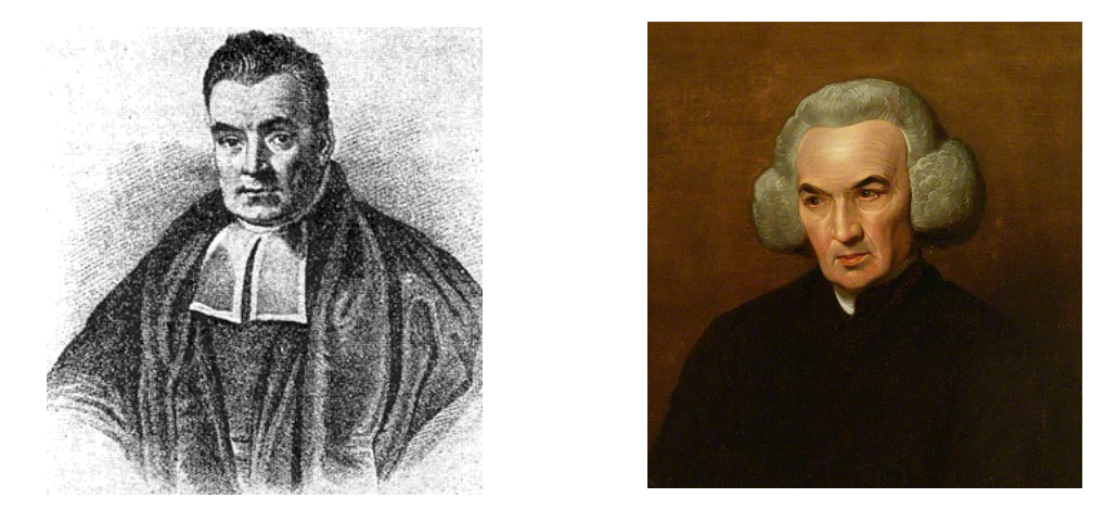
This work carried two essential advances. The primary was the derivation of Bayes’ theorem from conditional chance. The second was the introduction of the Beta distribution. Pierre Simon Laplace independently labored out the identical theorem and the Beta distribution, and likewise labored out lots of what we name chance idea right this moment.
Beta distributions begin with a coin toss metaphor, which have solely two potential outcomes, heads or tails. Therefore, the chance of ok successes in n trials is given by the binomial distribution (bi = “two”). This was identified already earlier than Bayes and Laplace got here to the scene. They took inspiration from the discrete binomial distribution and by making use of calculus, took it to the continual distribution land. They retained ok and n however referred to as them alpha (or variety of successes =ok) and beta(or variety of failures = n-k), which grew to become the form parameters of this new distribution, which they referred to as the “Beta” distribution.

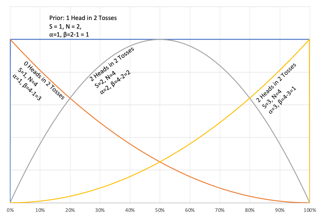
The superb factor about this distribution is that it’s form shifting in a method that matches our frequent sense. For those who have been to start out off your probabilistic inference by believing that you’ve got solely seen one success in two trials, then alpha = 1, beta = 2–1 = 1. The Beta(1,1) is definitely the Uniform Distribution. Altering alpha and beta modifications the distribution and helps us specific completely different beliefs.
Bayes instructed “with quite a lot of doubt” that the Uniform Distribution was the prior chance distribution to precise ignorance concerning the appropriate prior distribution. Laplace had no such hesitation and asserted this was the way in which to go after we felt every end result was equally seemingly. Additional, Laplace offered a succession rule which principally stated that we should use the imply of the distribution to put a chance on the subsequent coin touchdown heads (or the subsequent trial being thought-about successful).
Such was Laplace’s contribution in work Memoir on the Chance of the Causes of Occasions that most individuals within the West stopped specializing in chance idea believing there wasn’t way more to be superior there. The Russians didn’t get that memo, and they also continued to consider chance, producing elementary advances like Markov processes.
For our functions although, the subsequent huge leap in classical chance got here with the work of E. T. Jaynes, adopted by Ronald A. Howard. Earlier than we go there, did you discover an essential element? The x-axis of the graph above says “long-run fraction of heads”, and never “chance of heads.” This is a crucial element as a result of one can’t have a chance distribution on a chance — that’s non-interpretable. The place did this thought come from?
Like Bayes, Jaynes’ seminal work was by no means revealed in his lifetime. His scholar Larry Bretthorst revealed Chance Idea: The Logic of Science after his passing. Jaynes’ class notes have been an enormous affect within the work of my trainer, Ronald A. Howard, the co-founder of Choice Evaluation.
Jaynes launched the idea of a reasoning robotic which might use ideas of logic that we might agree with. He wrote within the e-book cited above: “In an effort to direct consideration to constructive issues and away from controversial irrelevancies, we will invent an imaginary being. Its mind is to be designed by us, in order that it causes in keeping with sure particular guidelines. These guidelines shall be deduced from easy desiderata which, it seems to us, could be fascinating in human brains; i.e. we expect {that a} rational individual, on discovering that they have been violating certainly one of these desiderata, would want to revise their pondering.”
“Our robotic goes to motive about propositions. As already indicated above, we will denote varied propositions by italicized capital letters, {A, B, C, and many others.}, and in the interim we should require that any proposition used should have, to the robotic, an unambiguous that means and should be of the easy, particular logical kind that should be both true or false.”
Jaynes’ robotic is the ancestor of Howard’s clairvoyant, an imaginary being that doesn’t perceive fashions however can reply factual questions concerning the future. The implication: we will solely place chances on distinctions which are clear, and haven’t a hint of uncertainty in them. In some early writings, you will notice the Beta distribution formulated on the “chance of heads.” A chance distribution on the “chance of heads” wouldn’t be interpretable in any significant method. Therefore, the edit that Ronald Howard offered in his seminal 1970 paper, Views on Inference, is to reframe the excellence because the long-run fraction of heads (or successes), a query that the clairvoyant can reply.
The beta distribution has a most attention-grabbing property. As we discover extra proof, we will merely replace alpha and beta, since they correspond to the variety of successes and the variety of failures, so as to acquire the up to date chance distribution on the excellence of curiosity. Right here is an easy instance of various configurations of alpha and beta (S = variety of successes, N = variety of tosses):
We are able to use this distribution to do our inference. I’ve ready a public area Google sheet (US model, India English model, India Kannada model) that you could play with after making a replica. I’ll use this sheet to clarify the remainder of the idea.
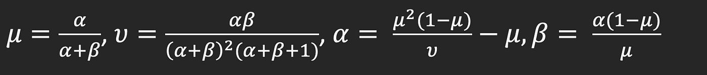
Keep in mind that we began with a distribution of non-conformance (4% to six%)? As an train for the reader, consult with the imply and variance of the Beta distribution and derive the formulae for alpha and beta utilizing imply and variance.
How do we discover the imply and variance of our prior evaluation? We assessed the next percentile / chance pairs from our mechanical engineering specialists:
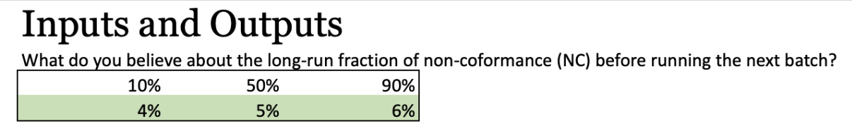
The interpretation of the above is that there’s solely a ten% likelihood of the non-conformance price being under 4%, and a ten% likelihood of being above 6%. There’s a 50–50 shot of being above or under 5%. A rule of thumb is to assign 25%/50%/25% to 10/50/ninetieth percentile. For those who’d wish to learn extra about this idea, see [1][2][3]. This shortcut makes it simple for us to compute the imply as:
Imply = 25% x 4% + 50% x 5% + 25% x 6% = 5%
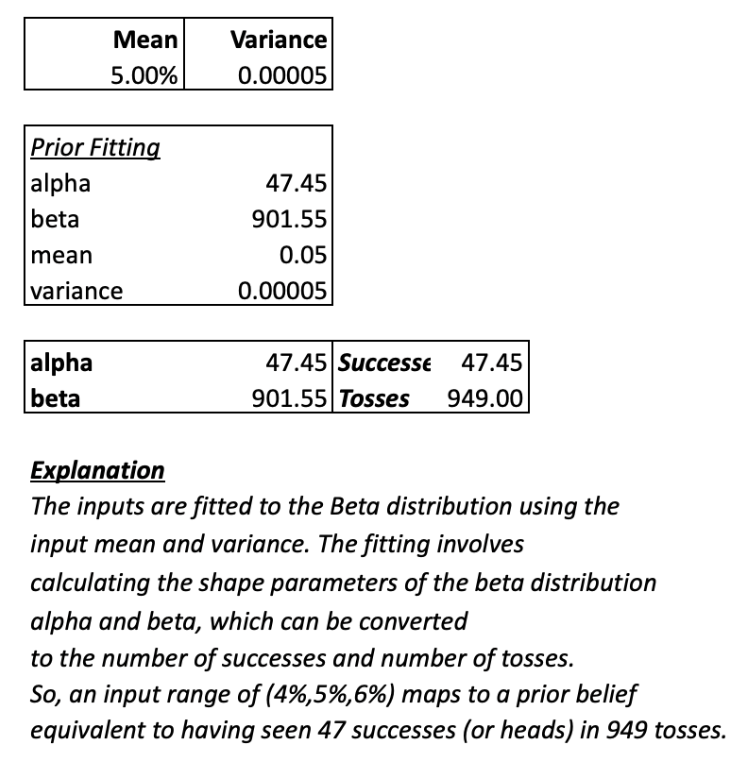
We are able to equally calculate the variance utilizing the usual system to yield the next alpha and beta form parameters.
As you may see, the worksheet reveals the equal variety of successes and tosses. Offering an enter of 4%-5%-6% as our prior perception is similar as saying, “we’ve a power of perception that’s equal to seeing 47 successes in 949 tosses.” This framing permits our specialists to cross-check whether or not 47 out of 949 tosses makes intuitive sense to them.
We are able to additionally discretize the fitted beta distribution and examine with the unique inputs, which is under.

Now that we’ve the prior, we will simply replace it with our observations. We ask the next query:

The brand new alpha (successes) and beta (failures) parameters are merely the sum of the earlier alpha with the brand new successes and the earlier beta with the brand new failures respectively. That is proven individually within the part under:

This may now be visualized in several methods. First, we will see the posterior distribution discretized and examine it with the inputs:
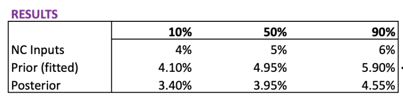
We see that the posterior distribution is left-shifted. We are able to additionally see this within the visualizations that observe:

First, by Laplace’s succession rule, we will reply the query: What’s the chance of the subsequent element being non-conforming?

This was arrived at by merely dividing the variety of posterior successes (posterior alpha) by the variety of posterior trials (posterior alpha + posterior beta), or the imply of the posterior distribution.
Since we’ve the posterior cumulative distribution, we will simply learn it to reply chance questions.
Subsequent, we’re inquisitive about realizing the chance of being under the goal non-conforming stage. We are able to reply this simply by studying the cumulative distribution operate in opposition to the goal stage. In our instance under, we will do the readout in opposition to each the prior and the posterior.
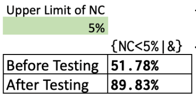
As we will see, our observations made us way more assured about being under the non-conforming stage. Word that this inference is sweet so far as it goes. One critique that may be leveled right here is that we’ve taken all the information at face worth and never discounted for the broader context through which this information might seem (as an illustration, what number of batches are we going to see over the yr?) Utilizing that data would lead us to introduce a posterior scale energy (a.ok.a. information scale energy) that will mood our inference from information.
Posterior scale energy or information scale energy might be regarded as the reply to the query: “what number of trials (successes) do I must see on this take a look at/batch to contemplate as one trial (success)?” The worksheet has set the information scale energy to 1 by default, which implies all the information is taken at face worth and absolutely used. The issue with that is that we will make up our thoughts too rapidly. An information scale energy of 10, which suggests that we are going to take each 10 trials as 1 trial and each 10 successes as 1 success, will instantly change our conclusion. As we will see under, the needle will barely transfer from the prior as we are actually treating the 30 successes in 1000 trials as 3 successes in 100 trials (dividing by 10).

Trying on the above, we are going to rapidly notice that we have to run extra batches so as to get extra confidence, accurately. Let’s say we ran 5 batches of 1000 parts every, and noticed the identical proportion as 30 successes over 1,000 trials — solely, we noticed 30 x 5 = 150 successes over 1,000 x 5 = 5,000 trials. We now see a near 90% confidence stage that we are going to be under the 5% goal non-conformance stage.

Now, a key query is: what’s a principled method of setting a knowledge scale energy? Let’s say we would like the forecast to be legitimate yearly. One precept we will use is the proportion of the manufactured batches used for inference out of the overall batches to be manufactured over the yr. Let’s say our plan was to fabricate 50 batches, and we haver used 5 batches for inference. Then, we will set our information scale energy to 50/5 (=10). One other strategy to interpret the information scale energy is that we’ve to dilute the information by 10 occasions so as to interpret it for the complete yr.
Let’s now flip to the ultimate forecasting query on working economics.
It is extremely simple to put an financial mannequin on high of the forecasting work we’ve already performed. By taking as inputs the worth and price of every element, the variety of batches to be processed in a yr, and the variety of parts in every batch, we will get a distribution of the variety of non-compliant parts by multiplying the overall parts manufactured (e.g. 50,000) by every merchandise within the NC posterior distribution that we produced within the prior part. We are able to then instantly calculate the loss distribution by multiplying the NC forecast by the price of every element. The working revenue can be calculated simply by calculating the online income of every compliant element and subtracting the lack of the non-compliant parts.
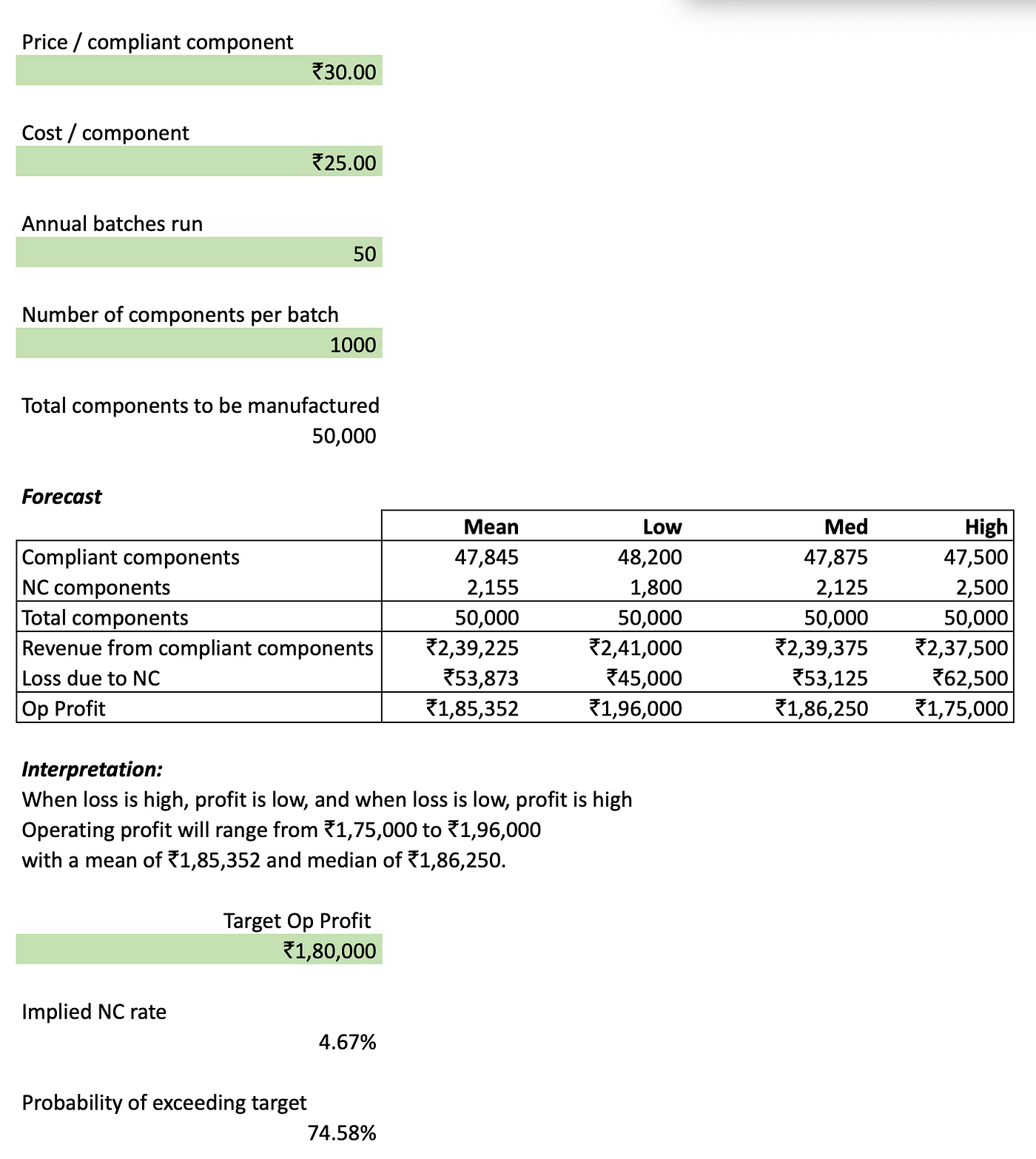
Additional, because the screenshot above reveals, we will calculate the chance of exceeding the goal working revenue, which is similar because the chance of being under the implied non-conformance price at that revenue goal, which we learn off from the cumulative density operate of the posterior (of non-conformance) within the earlier part.
This can be a easy mannequin to point out how we will get began utilizing chance in forecasting. There are limitations to this method, and one essential limitation is that we’re contemplating the worth, value, variety of batches run and the variety of parts produced as fastened. These may all be unsure, and when that occurs, the mannequin has to change into a bit extra subtle. The reader is referred to the Twister Diagram software to make extra subtle financial fashions that deal with multi-factor uncertainty.
Additional, the beta-binomial updating mannequin works provided that we assume stationarity within the course of of creating the components, that means there isn’t a drift. The sector of Statistical Course of Management[4] will get into drift, and that’s past the scope of this text.
—
Because of Dr. Brad Powley for reviewing this text, and to Anmol Mandhania for useful feedback. Errors are mine.
[1] Miller III, Allen C., and Thomas R. Rice. “Discrete approximations of chance distributions.” Administration science 29, no. 3 (1983): 352–362. See P8.
[2] McNamee, Peter, and John Nunzio Celona. Choice evaluation for the skilled. SmartOrg, Integrated, 2007. Free on-line PDF of e-book. See web page 36 in chapter: Encoding Possibilities.
[3] Howard, Ronald A. “The foundations of determination evaluation.” IEEE transactions on techniques science and cybernetics 4, no. 3 (1968): 211–219.
[4] “Out of the Disaster” Wheeler, D J & Chambers, D S (1992) Understanding Statistical Course of Management
