Causal Python: 3 Easy Methods to Soar-Begin Your Causal Inference Journey Right this moment | by Aleksander Molak | Sep, 2022

Study 3 methods for causal impact identification and implement them in Python with out shedding months, weeks or days for analysis

If you’re studying this you’ve most likely been in information science for some 2–5 years now. You will have most probably heard about causality earlier than, possibly even learn a e book or two on the subject, but in case you don’t really feel assured otherwise you’re lacking some readability on how one can seize these ideas and make them give you the results you want in observe with out shedding weeks and even months on analysis this put up is for you.

I’ve been in the same place! Sooner or later I learn extra virtually 1000 pages on causality together with books and analysis papers and I nonetheless didn’t have readability on how one can apply a few of these ideas in observe with out devoting weeks to implementation!

This weblog put up is right here that can assist you jump-start your causal inference journey tonight.

Let’s begin!

[Links to the notebook and the conda environment file are below]

On this put up we concentrate on causal inference. For the aim of this text, we’ll perceive causal inference as a strategy of estimating the causal impact of 1 variable on one other variable from observational information.

Causal impact estimate goals at capturing the power of (anticipated) change within the end result variable once we modify the worth of the therapy by one unit.

In observe, virtually any machine studying algorithm can be utilized for this objective, but normally we have to use these algorithms in a means that differs from the classical machine studying stream.

The primary problem (but not the one one) in estimating causal results from observational information comes from confounding. Confounder is a variable within the system of curiosity that produces a spurious relationship between the therapy and the result. Spurious relationship is a form of phantasm. Apparently, you’ll be able to observe spurious relationships not solely within the recorded information, but in addition in the true world. They type a powerful foundation for a lot of stereotypes and cognitive biases (however that’s for one more put up).

To be able to receive an unbiased estimate of the causal impact, we have to eliminate confounding. On the similar time, we must be cautious to not introduce confounding ourselves! This normally boils all the way down to controlling for the precise subset of variables in your evaluation. Not too small, not too giant. The artwork and science of choosing the right controls is a subject in itself.

Understanding it effectively is perhaps hampered by the truth that there’s plenty of complicated and inaccurate data on the topic on the market coming from numerous sources, together with even high-impact peer-reviewed journals (sic!). If this sounds fascinating to you, I’m going deeper on this matter in my upcoming e book on Causal Inference and Discovery in Python.

All for causality and Causal Machine Studying in Python?

Take a quick survey and let me know what you need to be taught: https://varieties.gle/xeU6V4yhB6cftNga6

[The survey closes on Oct 2, 2022; 3:00PM GMT]

Subscribe to the e-mail listing to get unique free content material on causality and updates on my causal e book: https://causalpython.io

Good information is that in some instances we are able to automate the method of selecting the best variables as controls. On this put up we are going to exhibit how one can use three totally different strategies to establish causal results from a graph:

1. Again-door criterion
2. Entrance-door criterion
3. Instrumental variables (IV)

The primary two strategies might be derived from a extra basic set of identification guidelines referred to as do-calculus that has been formulated by Judea Pearl and colleagues (e.g. Pearl, 2009).

The latter (IV) is a household of strategies very fashionable in econometrics. In response to Scott Cunningham (Cunningham, 2021) instrumental variable estimator was first launched as early as 1928 by Philip Wright (Wright, 1928).

Causal inference strategies require that particular assumptions are met. We received’t have house to debate all of them right here, however we’ll briefly evaluate a very powerful ones.

Causal graph

The primary basic assumption for causal inference as we perceive it right here is that we now have a causal graph encoding the relationships between the variables. Variables are encoded as nodes and relationships between them as directed edges. Course of the perimeters denotes the route of the causal affect.

Some strategies require that each one the variables are measured, some permit unmeasured variables in numerous configurations.

Again-door criterion

Again-door criterion requires that there are no hidden confounders in our information, i.e. there aren’t any variables that affect each the therapy and the result and are unobserved on the similar time. This assumption is perhaps troublesome to fulfill in among the real-world eventualities because it is perhaps troublesome to make sure that there isn’t any hidden variable that we’re unaware of and that influences the therapy and the result. That’s very true in case of very advanced programs (e.g. social, organic or medical contexts).

Entrance-door criterion

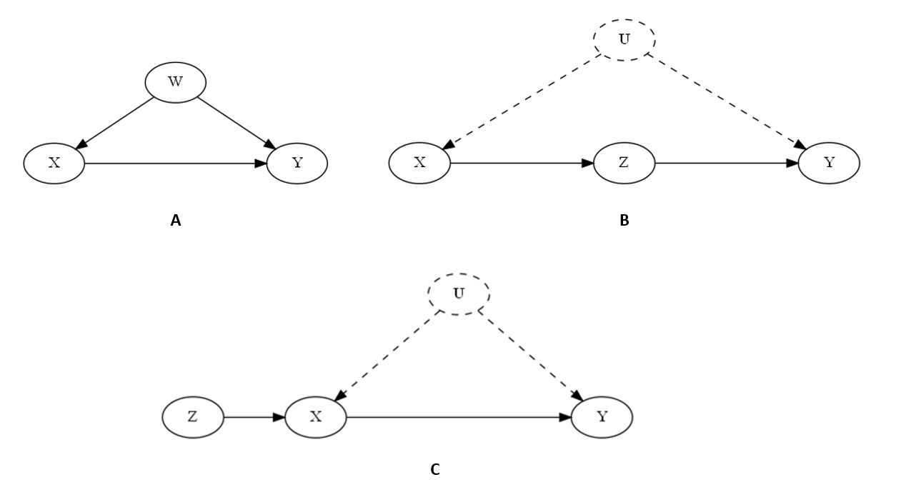
Entrance-door criterion permits for hidden confounding between the therapy and the result, but requires that the affect of the therapy on the result is absolutely mediated by one other variable that isn’t influenced by the hidden confounder. That’s mouthful! Be happy to take a sneak-peek at Determine 1(B) under to get some visible instinct.

Instrumental variables

Instrumental variables additionally permit for hidden confounding between the therapy and the result, but they require that there’s one other variable that’s related to the therapy, however not related to the result (neither instantly nor by way of a standard trigger; Hernán & Robbins, 2020).

Let’s check out Determine 1 to present some visible instinct to the assumptions we mentioned above.

DoWhy (Sharma & Kiciman, 2020) is a causal inference library that has began as a Microsoft’s open-source challenge and have been lately moved to an new challenge referred to as py-why. It’s developed by a workforce of seasoned researchers and builders and presents essentially the most complete set of functionalities amongst all Python causal libraries.

DoWhy has a few totally different APIs together with the primary object-oriented CausalModel API, high-level Pandas API and the brand new experimental GCM API. We’ll use the primary one on this put up.

The promise of DoWhy is that it’ll establish causal results within the graph routinely (assuming that they’re identifiable utilizing one of many three strategies we mentioned above). Which means that you would not have to look into the causal graph and determine your self which technique must be used (this could grow to be rather more troublesome with bigger graphs).

For the sake of this put up, we’ll generate three easy artificial datasets. Why artificial information? To make it tremendous clear for you what’s happening.

At each stage you’ll be capable of return to the information producing course of and see for your self what’s the true construction of the information set.

Let’s do it!

First, we import numpy and pandas. DoWhy operates natively on Pandas information frames, which is handy as a result of it makes it simple to establish your variables when constructing the mannequin and analyzing outcomes.

Subsequent, we generate three totally different information units. Word that structurally these datasets observe their counterparts in Determine 1. An vital factor to note is that in case of datasets 2 and three (their respective counterparts in Determine 1 being B and C) we didn’t embrace variable U within the information frames though it was used within the information producing course of. That is on objective as we’re mimicking the eventualities the place U is unobserved.

DoWhy’s foremost API presents a fantastic and intuitive option to carry out causal inference.

It consists of 4 steps:

1. Mannequin the issue
2. Discover the estimand
3. Estimate the impact
4. Refute the mannequin

On this article we’ll concentrate on the three first steps and run all of them for every of the three datasets.

Let’s begin with the mandatory imports after which bounce to the primary dataset.

Dataset 1 — Backdoor criterion

Let’s begin with dataset 1.

Step 1: Mannequin the issue

Step 1 has two sub-steps:

• Making a graph in a format that DoWhy can learn
• Instantiating the CausalModel object

In our examples we’ll use a graph language referred to as GML to outline the graphical construction of our datasets. Let’s begin!

GML syntax is slightly easy (not less than for easy graphs). If you wish to be taught extra about GML you are able to do it right here.

Now, let’s instantiate our mannequin object.

We handed the dataset and the graph to the constructor alongside therapy and end result variable names. That’s all we’d like!

Let’s visualize the mannequin to examine if the graph is what we anticipate it to be. You are able to do it through the use of model_1.view_model().

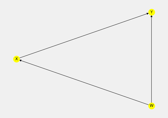
The graph appears to be like good! In Determine 2 We now have precisely the identical set of nodes and edges as in Determine 1A.

Step 2: Discover the estimand

Estimand denotes the amount that we need to estimate and is not the identical as estimate. You’ll be able to consider causal estimands as adjusted formulation that solely include the variables that we need to management for with the intention to receive unbiased causal estimates. Estimand isn’t a price nor a way of estimation, it’s a amount to be estimated.

Word that DoWhy has discovered only one estimand for dataset 1 — back-door. This is sensible, as a result of we don’t have any hidden confounding within the information neither is the impact of therapy mediated.

Let’s estimate the causal impact and examine if it’s what we might anticipate it to be.

Step 3: Estimate the impact

We referred to as the .estimate_effect() technique on the mannequin object and handed the estimand from the earlier step as an argument alongside the estimator technique title that we need to use. DoWhy presents many alternative estimators. For our objective linear regression is sweet sufficient.

How is the outcome? The estimate could be very near the true one. As you’ll be able to see in Code block 1, the true coefficient for X is 0.87 and the mannequin returned ~0.88¹.

Step 4: Refutation checks

Refutation checks are a means of implementing Karl Popper’s logic of falsifiability (Popper 1935; 1959) within the causal inference course of. This step is past the scope of this text. If you wish to see it rapidly in motion, you examine this pocket book, for an up-to-date listing of refutation checks accessible in DoWhy examine this web page.

Dataset 2 — Entrance-door criterion

Let’s repeat the entire course of with dataset 2.

Step 1: Mannequin the issue

Creating GML graphs by hand might be daunting. Let’s make it easier. We’ll outline an inventory of nodes and an inventory of edges and let two for-loops do the work for us.

Lovely. Let’s instantiate the mannequin.

I encourage you to examine in case your graph is as anticipated utilizing model_2.view_model(). You’ll be able to see it in motion within the pocket book accompanying this text (hyperlink under).

Step 2: Discover the estimand

We’re now prepared to seek out the estimand.

The one estimand discovered by DoWhy is front-door. That is anticipated for the graph we supplied. Let’s examine the estimated impact.

Step 3: Estimate the impact

The method is just about equivalent to what we’ve seen earlier than. Word that we’ve modified the method_name to frontdoor.two_stage_regression.

We see that the estimated impact is ~0.66. What’s the anticipated true impact? We are able to compute it because of Sewall Wright, a son of Philip Wright (sic!) that we talked about earlier within the context of instrumental variables. In response to Judea Pearl (Pearl, 2019), Sewall Wright was the primary who launched path evaluation — a way of assessing the causal impact power in linear programs (Wright, 1920). To get a real causal coefficient we have to multiply all of the coefficients on the best way between the therapy and the result.

In our case, the causal affect goes like this: X → Z → Y. We take the coefficient of X within the method for Z and the coefficient for Z within the method for Y and multiply them collectively. Subsequently, the true causal impact is 0.78 x 0.87 = 0.6786. DoWhy did a fairly good job²!

Dataset 3 — Instrumental variable

It’s virtually time to say goodbye. Earlier than we achieve this, let’s undergo the entire 4-step course of for the final time and see the instrumental variable approach in motion!

Step 1: Mannequin the issue

This time we’ll additionally use for-loops to automate the GML graph definition creation.

Let’s instantiate the CausalModel object.

Once more, I encourage you to make use of model_3.view_model(). Generally it’s very simple to make a mistake in your graph and the results will normally be detrimental to your estimate.

Step 2: Discover the estimand

DoWhy accurately acknowledged that the causal impact for dataset 3 might be recognized utilizing the instrumental variable approach. Let’s estimate the impact!

Step 3: Estimate the impact