YOLOv7: A deep dive into the present state-of-the-art for object detection | by Chris Hughes & Bernat Puig Camps

All the things it is advisable to know to make use of YOLOv7 in customized coaching scripts

This text was co-authored by Chris Hughes & Bernat Puig Camps

Shortly after its publication, YOLOv7 is the quickest and most correct real-time object detection mannequin for laptop imaginative and prescient duties. The official paper demonstrates how this improved structure surpasses all earlier YOLO variations — in addition to all different object detection fashions — when it comes to each pace and accuracy on the MS COCO dataset; attaining this efficiency with out using any pretrained weights. Moreover, following the entire controversy across the naming conventions of earlier YOLO fashions, as YOLOv7 was launched by the identical authors that developed Scaled-YOLOv4, the machine studying neighborhood appears completely happy to simply accept this as the following iteration of the ‘official’ YOLO household!

On the level that YOLOv7 was launched, we — as a part of Microsoft’s Knowledge & AI Service Line — had been partway by means of a difficult object-detection primarily based buyer undertaking, in a website drastically completely different to COCO. Evidently, each ourselves and the client had been very excited on the prospect of making use of YOLOv7 to our downside. Sadly, when utilizing the out-of-the-box settings, the outcomes had been … let’s simply say, not nice.

After studying the official paper, we discovered that, while it presents a complete overview on the architectural adjustments, it omits many particulars round how the mannequin was skilled; for instance, which knowledge augmentation strategies had been utilized, and the way the loss operate measures that the mannequin is doing a very good job! To grasp these technicalities, we determined to debug the code straight. Nevertheless, because the YOLOv7 repository is a modified fork of the YOLOR codebase — which itself is a fork of YOLOv5 — we discovered that it contains lots of complicated performance, a lot of which isn’t wanted when simply coaching a mannequin; for instance, having the ability to specify customized architectures in Yaml format and have these translated into PyTorch fashions. Moreover, the codebase accommodates many customized elements which have been applied from scratch — comparable to a multi-GPU coaching loop, a number of knowledge augmentations, samplers to protect dataloader staff, and a number of studying price schedulers — lots of which are actually obtainable in PyTorch, or different libraries. Because of this, there was lots of code to dissect; it took us a very long time to grasp how every part labored, in addition to the intricacies of the coaching loop which contribute to the mannequin’s glorious efficiency! Ultimately, with this understanding, we had been in a position to arrange our coaching recipe to acquire constantly good outcomes on our process.

On this article, we intend to take a sensible strategy in demonstrating how you can prepare YOLOv7 fashions in customized coaching scripts, in addition to exploring areas comparable to knowledge augmentation strategies, how you can choose and modify anchor containers, and demystifying how the loss operate works; (hopefully!) enabling you to construct up an instinct of what’s prone to work properly in your personal issues. Because the YOLOv7 structure is properly described intimately within the official paper, in addition to in lots of different sources, we’re not going to cowl this right here. As an alternative, we intend to give attention to the entire different particulars which, while contribute to YOLOv7’s efficiency, are not lined within the paper. This tends to be information which has been accrued over a number of variations of YOLO fashions however could be extremely troublesome to trace down for somebody simply coming into the sphere.

For instance these ideas, we will be utilizing our personal implementation of YOLOv7, which utilises the official pretrained weights, however has been written with modularity and readability in thoughts. This undertaking initially began as an train for us to enhance our understanding of how YOLOv7 works underneath the hood — with a purpose to higher perceive how you can apply it — however after efficiently utilizing it on just a few completely different duties, we’ve got determined to make it publicly obtainable. While we might advocate utilizing the official implementation should you want to precisely reproduce the revealed outcomes on COCO, we discover that this implementation is extra versatile to use, and prolong, to customized domains. Hopefully, this implementation will present a clear and clear start line for anybody wishing to experiment with YOLOv7 in their very own customized coaching scripts, in addition to offering extra transparency across the strategies that had been used throughout coaching within the authentic implementation.

On this article, we will cowl:

Exploring the entire particulars alongside the way in which, comparable to:

Tl;dr: Should you simply wish to see some working code that you should use straight, the entire code required to copy this publish is obtainable as a pocket book right here. While code snippets are used all through the article, that is primarily for aesthetic functions, please defer to the pocket book, and the repo for working code.

We wish to thank British Airways, for with out their constantly delayed flights, this publish would in all probability not have occurred.

First, let’s check out how you can load our dataset within the format that YOLOv7 expects.

Choosing a dataset

All through this text, we will use the Kaggle automobiles object detection dataset; nevertheless, as our purpose is to reveal how YOLOv7 could be utilized to any downside, that is actually the least vital a part of this work. Moreover, as the pictures are fairly much like COCO, it would allow us to experiment with a pretrained mannequin earlier than we do any coaching.

The annotations for this dataset are within the type of a .csv file, which associates the picture identify with the corresponding annotations; the place every row represents one bounding field. While there are round 1000 photos within the coaching set, solely these with annotations are included on this file.

We are able to view the format of this by loading it right into a pandas DataFrame.

As it’s not normally the case that each one photos in our dataset comprise cases of the objects that we are attempting to detect, we might additionally like to incorporate some photos that don’t comprise automobiles. To do that, we will outline a operate to load the annotations which additionally contains 100 ‘destructive’ photos. Moreover, because the designated take a look at set is unlabelled, let’s randomly take 20% of those photos to make use of as our validation set.

# https://github.com/Chris-hughes10/Yolov7-training/blob/important/examples/train_cars.py
import pandas as pd
import random
def load_cars_df(annotations_file_path, images_path):
all_images = sorted(set([p.parts[-1] for p in images_path.iterdir()]))
image_id_to_image = {i: im for i, im in enumerate(all_images)}
image_to_image_id = {v: ok for ok, v, in image_id_to_image.objects()}
annotations_df = pd.read_csv(annotations_file_path)
annotations_df.loc[:, "class_name"] = "automobile"
annotations_df.loc[:, "has_annotation"] = True
# add 100 empty photos to the dataset
empty_images = sorted(set(all_images) - set(annotations_df.picture.distinctive()))
non_annotated_df = pd.DataFrame(record(empty_images)[:100], columns=["image"])
non_annotated_df.loc[:, "has_annotation"] = False
non_annotated_df.loc[:, "class_name"] = "background"
df = pd.concat((annotations_df, non_annotated_df))
class_id_to_label = dict(
enumerate(df.question("has_annotation == True").class_name.distinctive())
)
class_label_to_id = {v: ok for ok, v in class_id_to_label.objects()}
df["image_id"] = df.picture.map(image_to_image_id)
df["class_id"] = df.class_name.map(class_label_to_id)
file_names = tuple(df.picture.distinctive())
random.seed(42)
validation_files = set(random.pattern(file_names, int(len(df) * 0.2)))
train_df = df[~df.image.isin(validation_files)]
valid_df = df[df.image.isin(validation_files)]
lookups = {
"image_id_to_image": image_id_to_image,
"image_to_image_id": image_to_image_id,
"class_id_to_label": class_id_to_label,
"class_label_to_id": class_label_to_id,
}
return train_df, valid_df, lookups

We are able to now use this operate to load our knowledge:

To make it simpler to affiliate predictions with a picture, we’ve got assigned every picture a novel id; on this case it’s simply an incrementing integer rely. Moreover, we’ve got added an integer worth to symbolize the courses that we wish to detect, which is a single class — ‘automobile’ — on this case.

Typically, object detection fashions reserve 0 because the background class, so class labels ought to begin from 1. That is not the case for YOLOv7, so we begin our class encoding from 0. For photos that don’t comprise a automobile, we don’t require a category id. We are able to verify that that is the case by inspecting the lookups returned by our operate.

Lastly, let’s see the variety of photos in every class for our coaching and validation units. As a picture can have a number of annotations, we have to ensure that we account for this when calculating our counts:

Create a Dataset Adaptor

Normally, at this level, we might create a PyTorch dataset particular to the mannequin that we will be coaching.

Nevertheless, we frequently use the sample of first making a dataset ‘adaptor’ class, with the only accountability of wrapping the underlying knowledge sources and loading this appropriately. This fashion, we will simply change out adaptors when utilizing completely different datasets, with out altering any pre-processing logic which is restricted to the mannequin that we’re coaching.

Due to this fact, let’s focus for now on making a CarsDatasetAdaptor class, which converts the precise uncooked dataset format into a picture and corresponding annotations. Moreover, let’s load the picture id that we assigned, in addition to the peak and width of our picture, as they could be helpful to us afterward.

An implementation of that is introduced beneath:

# https://github.com/Chris-hughes10/Yolov7-training/blob/important/examples/train_cars.py
from torch.utils.knowledge import Dataset
class CarsDatasetAdaptor(Dataset):
def __init__(
self,
images_dir_path,
annotations_dataframe,
transforms=None,
):
self.images_dir_path = Path(images_dir_path)
self.annotations_df = annotations_dataframe
self.transforms = transforms
self.image_idx_to_image_id = {
idx: image_id
for idx, image_id in enumerate(self.annotations_df.image_id.distinctive())
}
self.image_id_to_image_idx = {
v: ok for ok, v, in self.image_idx_to_image_id.objects()
}
def __len__(self) -> int:
return len(self.image_idx_to_image_id)
def __getitem__(self, index):
image_id = self.image_idx_to_image_id[index]
image_info = self.annotations_df[self.annotations_df.image_id == image_id]
file_name = image_info.picture.values[0]
assert image_id == image_info.image_id.values[0]
picture = Picture.open(self.images_dir_path / file_name).convert("RGB")
picture = np.array(picture)
image_hw = picture.form[:2]
if image_info.has_annotation.any():
xyxy_bboxes = image_info[["xmin", "ymin", "xmax", "ymax"]].values
class_ids = image_info["class_id"].values
else:
xyxy_bboxes = np.array([])
class_ids = np.array([])
if self.transforms is just not None:
remodeled = self.transforms(
picture=picture, bboxes=xyxy_bboxes, labels=class_ids
)
picture = remodeled["image"]
xyxy_bboxes = np.array(remodeled["bboxes"])
class_ids = np.array(remodeled["labels"])
return picture, xyxy_bboxes, class_ids, image_id, image_hw

Discover that, for our background photos, we’re simply returning an empty array for our bounding containers and sophistication ids.

Utilizing this, we will verify that the size of our dataset is identical as the whole variety of coaching photos that we calculated earlier.

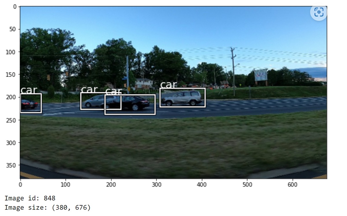
Now, we will use this to visualise a few of our photos, as demonstrated beneath:

Create a YOLOv7 dataset

Now that we’ve got created our dataset adaptor, let’s create a dataset which preprocesses our inputs into the format required by YOLOv7; these steps ought to stay the identical whatever the adaptor that we’re utilizing.

An implementation of that is introduced beneath:

# https://github.com/Chris-hughes10/Yolov7-training/blob/important/yolov7/dataset.py
class Yolov7Dataset(Dataset):
"""
A dataset which takes an object detection dataset returning (picture, containers, courses, image_id, image_hw)
and applies the mandatory preprocessing steps as required by Yolov7 fashions.
By default, this class expects the picture, containers (N, 4) and courses (N,) to be numpy arrays,
with the containers in (x1,y1,x2,y2) format, however this behaviour could be modified by
overriding the `load_from_dataset` methodology.
"""
def __init__(self, dataset, transforms=None):
self.ds = dataset
self.transforms = transforms
def __len__(self):
return len(self.ds)
def load_from_dataset(self, index):
picture, containers, courses, image_id, form = self.ds[index]
return picture, containers, courses, image_id, form
def __getitem__(self, index):
picture, containers, courses, image_id, original_image_size = self.load_from_dataset(
index
)
if self.transforms is just not None:
remodeled = self.transforms(picture=picture, bboxes=containers, labels=courses)
picture = remodeled["image"]
containers = np.array(remodeled["bboxes"])
courses = np.array(remodeled["labels"])
picture = picture / 255  # 0 - 1 vary
if len(containers) != 0:
# filter containers with 0 space in any dimension
valid_boxes = (containers[:, 2] > containers[:, 0]) & (containers[:, 3] > containers[:, 1])
containers = containers[valid_boxes]
courses = courses[valid_boxes]
containers = torchvision.ops.box_convert(
torch.as_tensor(containers, dtype=torch.float32), "xyxy", "cxcywh"
)
containers[:, [1, 3]] /= picture.form[0]  # normalized top 0-1
containers[:, [0, 2]] /= picture.form[1]  # normalized width 0-1
courses = np.expand_dims(courses, 1)
labels_out = torch.hstack(
(
torch.zeros((len(containers), 1)),
torch.as_tensor(courses, dtype=torch.float32),
containers,
)
)
else:
labels_out = torch.zeros((0, 6))
attempt:
if len(image_id) > 0:
image_id_tensor = torch.as_tensor([])
besides TypeError:
image_id_tensor = torch.as_tensor(image_id)
return (
torch.as_tensor(picture.transpose(2, 0, 1), dtype=torch.float32),
labels_out,
image_id_tensor,
torch.as_tensor(original_image_size),
)

Let’s wrap our knowledge adaptor utilizing this dataset and examine a number of the outputs:

As we haven’t outlined any transforms, the output is basically the identical, with the primary exception being that the containers are actually in normalized cxcywh format and all of our outputs have been transformed into tensors. Word that cx, cy stands for middle x and y and it signifies that the coordinates correspond to the centre of the field.

One factor to notice is that our labels take the shape [0, class_id, ncx, ncy, nw, nh]. The zero area in the beginning of the tensor can be utilised by the collate operate afterward.

Transforms

Now, let’s outline some transforms! For this, we will use the wonderful Albumentations library, which supplies many choices for reworking each photos and bounding containers.

While the transforms that we choose will largely be area particular, right here, we will ‘s outline comparable transforms to these used within the authentic implementation.

These are:

• Resize the picture to the given enter (a number of of 640) while sustaining the facet ratio
• If the picture is just not sq., apply padding. For this, we will comply with the paper in utilizing a gray padding, that is an arbitrary selection.

Throughout coaching:

We are able to use the next operate to create these transforms as demonstrated beneath:

# https://github.com/Chris-hughes10/Yolov7-training/blob/important/yolov7/dataset.py
def create_yolov7_transforms(
image_size=(640, 640),
coaching=False,
training_transforms=(A.HorizontalFlip(p=0.5),),
):
transforms = [
A.LongestMaxSize(max(image_size)),
A.PadIfNeeded(
image_size[0],
image_size[1],
border_mode=0,
worth=(114, 114, 114),
),
]
if coaching:
transforms.prolong(training_transforms)
return A.Compose(
transforms,
bbox_params=A.BboxParams(format="pascal_voc", label_fields=["labels"]),
)

Now, let’s re-create our dataset, this time passing the default transforms that can be used throughout analysis. For our goal picture measurement, we will use 640 which is the worth that the smaller YOLOv7 fashions had been skilled on. Basically, we will choose any a number of of 8 for this.

Utilizing these transforms, we will see that our picture has been resized to our goal measurement and padding has been utilized. The explanation that padding is used is in order that we will keep the facet ratio of the objects within the photos, however have a typical measurement for photos in our dataset; enabling us to batch them effectively!

Now that we’ve got explored how you can load and put together our knowledge, let’s transfer on to check out how we will leverage a pretrained mannequin to make some predictions!

Loading the mannequin

In order that we will perceive how you can interface with the mannequin, let’s load a pretrained checkpoint and use this for inference on some photos in our dataset. As this checkpoint was skilled on COCO, which accommodates photos of automobiles, we will assume that the mannequin ought to carry out reasonably properly on this process out of the field. To see the fashions which might be obtainable, we will import the AVAILABLE_MODELS variable.

Right here, we will see that the obtainable fashions are the architectures outlined within the authentic paper. Let’s create the usual yolov7 mannequin, utilizing the create_yolov7_model operate.

Now, let’s check out the mannequin’s predictions. The ahead cross by means of the mannequin will return the uncooked function maps given by the FPN heads, to transform these into significant predictions, we will use the postprocess methodology.

Inspecting the form, we will see that the mannequin has made 25,200 predictions! Every prediction has an related tensor of size 6 — the entries correspond to the bounding field coordinates in xyxy format, a confidence rating, and a category index.

Typically, object detection fashions are likely to make lots of comparable, overlapping predictions. While there are various methods of coping with this, within the authentic paper, the authors used non-maximum-suppression (NMS) to unravel this downside. We are able to apply NMS, in addition to a secondary spherical of confidence thresholding, utilizing the operate beneath. As well as, throughout postprocessing, we frequently wish to filter our any predictions with a confidence stage beneath a predefined threshold, let’s enhance our confidence threshold right here.

# https://github.com/Chris-hughes10/Yolov7-training/blob/important/yolov7/coach.py
def filter_eval_predictions(
predictions: Record[Tensor],
confidence_threshold: float = 0.2,
nms_threshold: float = 0.65,
) -> Record[Tensor]:
nms_preds = []
for pred in predictions:
pred = pred[pred[:, 4] > confidence_threshold]
nms_idx = torchvision.ops.batched_nms(
containers=pred[:, :4],
scores=pred[:, 4],
idxs=pred[:, 5],
iou_threshold=nms_threshold,
)
nms_preds.append(pred[nms_idx])
return nms_preds

After making use of NMS, we will see that now we solely have a single prediction for this picture. Let’s visualise how this appears:

We are able to see that this appears fairly good! The prediction from the mannequin is definitely tighter across the automobile than the bottom reality!

Now that we’ve got our prediction, the one factor to notice is that the bounding field is relative to the resized picture measurement. To scale our predictions again to the unique picture measurement, we will use the next operate:

# https://github.com/Chris-hughes10/Yolov7-training/blob/important/yolov7/coach.py
def scale_bboxes_to_original_image_size(
xyxy_boxes, resized_hw, original_hw, is_padded=True
):
scaled_boxes = xyxy_boxes.clone()
scale_ratio = resized_hw[0] / original_hw[0], resized_hw[1] / original_hw[1]
if is_padded:
# take away padding
pad_scale = min(scale_ratio)
padding = (resized_hw[1] - original_hw[1] * pad_scale) / 2, (
resized_hw[0] - original_hw[0] * pad_scale
) / 2
scaled_boxes[:, [0, 2]] -= padding[0]  # x padding
scaled_boxes[:, [1, 3]] -= padding[1]  # y padding
scale_ratio = (pad_scale, pad_scale)
scaled_boxes[:, [0, 2]] /= scale_ratio[1]
scaled_boxes[:, [1, 3]] /= scale_ratio[0]
# Clip bounding xyxy bounding containers to picture form (top, width)
scaled_boxes[:, 0].clamp_(0, original_hw[1])  # x1
scaled_boxes[:, 1].clamp_(0, original_hw[0])  # y1
scaled_boxes[:, 2].clamp_(0, original_hw[1])  # x2
scaled_boxes[:, 3].clamp_(0, original_hw[0])  # y2
return scaled_boxes

Earlier than we will begin coaching, along with a mannequin structure, we want a loss operate which can allow us to measure how properly our mannequin is performing; so as to have the ability to replace our parameters. Since Object Detection is a troublesome downside to show a mannequin, the loss capabilities of such fashions are normally fairly complicated and YOLOv7 is just not an exception. Right here, we will do our greatest for example the intuitions behind it to facilitate its understanding.

Earlier than we will delve deeper into the precise loss operate, let’s cowl just a few background ideas that we have to perceive.

Anchor containers

One of many important difficulties of object detection is outputting detection containers. That’s, how can we prepare a mannequin to create a bounding field and localize it accurately in a picture?

There are just a few completely different approaches, however the YOLOv7 household is what we name an anchor-based mannequin. In these fashions, the overall philosophy is to first create plenty of potential bounding containers, then choose essentially the most promising choices to match to our goal objects; barely transferring and resizing them as mandatory to acquire the very best match.

The fundamental concept is that we draw a grid on prime of every picture and, at every grid intersection (anchor level), generate candidate containers (anchor containers) primarily based on plenty of anchor sizes. That’s, the identical set of containers is repeated at every anchor level. This fashion, the duty that mannequin has to be taught, barely relocating and resizing these containers, is less complicated than producing containers from scratch.

Nevertheless, one subject with this strategy is that our goal, floor reality, containers can vary in measurement — from tiny to very large! Due to this fact, it’s normally not attainable to outline a single set of anchor sizes that may be matched to all targets. For that reason, anchor-based mannequin architectures normally make use of a Function-Pyramid-Community (FPN) to help with this; which is the case with YOLOv7.

Function Pyramid Networks (FPN)

The principle concept behind FPNs (launched in Function Pyramid Networks for Object Detection) is to leverage the character of convolutional layers — which cut back the scale of the function area and enhance the protection of every function within the preliminary picture — to output predictions at completely different scales¹. FPNs are normally applied as a stack of convolutional layers, as we will see by inspecting the detection head of our YOLOv7 mannequin.

While we might merely take the outputs of the ultimate layer as predictions, because the deeper convolutional layers implicitly utilise the data from earlier layers to be taught extra high-level options, they don’t have entry to the data of how you can detect the lower-level options contained in earlier layers; this can lead to poor efficiency when detecting smaller objects.

For that reason, a top-down pathway and lateral connections are added to the common bottom-up pathway (regular movement of a convolution layer). The highest-down pathway hallucinates greater decision options by upsampling spatially coarser, however semantically stronger, function maps from greater pyramid ranges. Then, these options are enhanced with options from the bottom-up pathway by means of the lateral connections. The underside-up function map is of lower-level semantics, however its activations are extra precisely localized because it was subsampled fewer times¹.

In abstract, FPNs present semantically robust options at a number of scales which make them extraordinarily properly suited to object detection. The connections that YOLOv7 implements in its FPN are illustrated within the determine beneath:

Right here, we will see that we’ve got a “Regular mannequin” and a “Mannequin with auxiliary head”. It is because a number of the bigger fashions within the YOLOv7 household use deep supervision when coaching; that’s, they leverage the outputs of deeper layers within the loss with a purpose to try to higher be taught the duty. We will discover this additional afterward.

From the picture, we will see that every layer within the FPN (also called every FPN head), has a function scale that’s half the scale of the earlier one (the dimensions is identical for every Lead head and its corresponding Aux head). This may be understood as every subsequent FPN head “seeing” object scales twice as large because the earlier one. We are able to leverage that by assigning grids with completely different strides (grid cell aspect measurement), and proportional anchor sizes, to every FPN head.

As an example, the anchor configuration for the essential yolov7 mannequin appears like this:

As we will see, we’ve got anchor field sizes and grids that cowl fully completely different scales: from tiny objects to things that may occupy the entire picture.

Now, that we perceive these concepts conceptually, let’s check out the FPN outputs that come out of our mannequin, which is what can be used to calculate our loss.

¹ These sections had been straight taken from the authentic FPN paper as we felt that no additional clarification was wanted.

Breaking down the FPN outputs

Recall that, once we made our predictions earlier, we used the mannequin’s postprocess methodology to transform the uncooked FPN outputs into usable bounding containers. Now that we perceive the instinct behind what the FPN is attempting to do, let’s examine these uncooked outputs.

The outputs of our mannequin are all the time a Record[Tensor], the place every element corresponds to a head of the FPN. For fashions that use Deep Supervision, the Aux Head outputs come after the Lead Head outputs (all the time the identical variety of every, each side of the pair ordered equally). For the remainder, together with the one we’re utilizing right here, solely the Lead Head outputs are current.

Inspecting the form of every FPN output, we will see that every one has the next dimensions:

[n_images, n_anchor_sizes, n_grid_rows, n_grid_cols, n_features]

the place:

• n_images — The variety of photos within the batch (batch measurement).
• n_anchor_sizes – The anchor sizes related to the top (normally 3).
• n_grid_rows – The variety of anchors vertically, img_height / stride.
• n_grid_cols – The variety of anchors horizontally, img_width / stride.
• n_features – 5 + num_classes
  – cx – Horizontal correction for the anchor field centre.
  – cy – Vertical correction for the anchor field centre.
  – w – Width correction for the anchor field.
  – h – Top correction for the anchor field.
  – obj_score – Rating proportional to the chance of an object being contained contained in the anchor field.
  – cls_score – One per class, rating proportional to the chance of that being the category of the item.

When these outputs are mapped into helpful predictions throughout post-processing, we apply the next operations:

• cx, cy : closing = 2 * sigmoid(preliminary) - 0.5
  [(−∞, ∞), (−∞, ∞)] → [(−0.5, 1.5), (−0.5, 1.5)]
  – The mannequin can solely transfer the anchor centre from 0.5 cell behind to 1.5 cells ahead. Word that for the loss (i.e., once we prepare) we use grid coordinates.
• w, h : closing = (2 * sigmoid(preliminary)**2
  [(−∞, ∞), (−∞, ∞)] → [(0, 4), (0, 4)]
  – The mannequin could make the anchor field arbitrarily smaller however at most 4 instances greater. Bigger objects, outdoors of this vary, have to be predicted by the following FPN head.
• obj_score : closing = sigmoid(preliminary)
  (−∞, ∞) → (0, 1)
  – Makes certain the rating is mapped to a chance.
• cls_score : closing = sigmoid(preliminary)
  (−∞, ∞) → (0, 1)
  – Makes certain the rating is mapped to a chance.

Middle Priors

Now, it’s straightforward to see that if we put 3 anchor containers in every anchor level of every of the grids, we find yourself with lots of containers: 3*80*80 + 3*40*40 + 3*20*20=25200 for every 640x640px picture to be actual! The problem is that almost all of those predictions aren’t going to comprise an object, which we classify as ‘background’. Relying on the sequence of operations that we have to apply to every prediction, computations can simply stack up and decelerate the coaching!

To make the issue cheaper computationally, the YOLOv7 loss finds first the anchor containers which might be prone to match every goal field and treats them in another way — these are generally known as the middle prior anchor containers. This course of is utilized at every FPN head, for every goal field, throughout all photos in batch without delay.

Every anchor — that are the coordinates in our grid — defines a grid cell; the place we contemplate the anchor to be on the prime left of its corresponding grid cell. Subsequently, every cell (besides cells on the border) has 4 adjoining cells (prime, backside, left, proper). Every goal field, for every FPN head, lies someplace inside a grid cell. Think about that we’ve got the next grid, and the centre of a goal field is represented by a *:

Based mostly on the way in which the mannequin is designed and skilled, the x and y corrections that it might output are within the vary of [-0.5, 1.5] grid cells. Thus, solely a subset of the closest anchor containers will have the ability to match the goal centre. We choose a few of these anchor containers to symbolize the middle prior for the goal field.

• For the Lead Heads, we use a high-quality Middle Prior, which is a extra focused choice. That is comprised of 3 anchors per head: the anchor related the cell containing the goal field centre, alongside the anchors for the two closest grid cells to the goal field centre. Within the diagram, the Middle Prior anchors are marked with an X.

• For the Auxiliary Heads (for fashions that use deep supervision), we use a coarse Middle Prior, which is a much less focused choice. That is comprised of 5 anchors per head: the anchor of the cell containing the goal field centre, alongside all 4 adjoining grid cells.

The reasoning behind this high-quality and coarse distinction is that the training means of Auxiliary Heads is decrease than that of the Lead Heads, as a result of the Lead Heads are deeper within the community. Thus, we attempt to keep away from limiting an excessive amount of from the place the Auxiliary Head can be taught to verify we don’t lose precious data.

Equally to the coordinate corrections, the mannequin can solely apply a multiplicative modifier to the width and top of every anchor field within the interval [0, 4]. Which means that, at most, it might make the perimeters of the anchor containers 4 instances greater. Due to this fact, from the anchor containers chosen as Middle Prior, we filter these which might be both 4 instances greater or smaller than the goal field.

In abstract, the Middle Prior is comprised by the anchor containers whose anchor is shut sufficient to the goal field centre and whose sides aren’t too far off from the goal field aspect measurement.

Optimum Transport Project

One of many difficulties when evaluating object detection fashions is having the ability to match predicted containers to focus on containers with a purpose to quantify if the mannequin is doing a very good job or not.

The best strategy is to outline an Intersection over Union (IoU) threshold and resolve primarily based on that. Whereas this typically works, it turns into problematic when there are occlusions, ambiguity or when a number of objects are very shut collectively. Optimum Transport Project (OTA) goals to unravel a few of these issues by contemplating label task as a world optimization downside for every picture.

The principle instinct consists in contemplating every goal field a provider of ok constructive label assignments and every predicted field a demander of both one constructive label task or one background task. ok is dynamic and is determined by every goal field. Then, transporting one constructive label task from goal field to predicted field has a value primarily based on classification and regression. Lastly, the purpose is to discover a transportation plan (label task) that minimizes the whole price over the picture.

This may be completed utilizing an off-the-shelf solver, however YOLOv7 implements simOTA (launched within the YOLOX paper), a simplified model of the OTA downside. With the purpose of decreasing the computational price of label task, it assigns the 𝑘 predicted containers for every goal which have the bottom transportation price as an alternative of fixing the worldwide downside. The Middle Prior containers are used as candidates for this course of.

This helps us to additional filter the quantity of mannequin outputs that may doubtlessly be matched to a floor reality goal.

YOLOv7 Loss algorithm

Now that we’ve got launched essentially the most difficult items used within the YOLOv7 loss calculation, we will break down the algorithm used into the next steps:

1. For every FPN head (or every FPN head and Aux FPN head pair if Aux heads used):

• Discover the Middle Prior anchor containers.
• Refine the candidate choice by means of the simOTA algorithm. All the time use lead FPN heads for this.
• Get hold of the objectness loss rating utilizing Binary Cross Entropy Loss between the expected objectness chance and the Full Intersection over Union (CIoU) with the matched goal as floor reality. If there aren’t any matches, that is 0.
• If there are any chosen anchor field candidates, additionally calculate (in any other case they’re simply 0):
  – The field (or regression) loss, outlined because the imply(1 - CIoU) between all candidate anchor containers and their matched goal.
  – The classification loss, utilizing Binary Cross Entropy Loss between the expected class possibilities for every anchor field and a one-hot encoded vector of the true class of the matched goal.
• If mannequin makes use of auxiliary heads, add every element obtained from the aux head to the corresponding important loss element (i.e., x = x + aux_wt*aux_x). The contribution weight (aux_wt) is outlined by a predefined hyperparameter.
• Multiply the objectness loss by the corresponding FPN head weight (predefined hyperparameter).

2. Multiply every loss element (objectness, classification, regression) by their contribution weight (predefined hyperparameter).

3. Sum the already weighted loss elements.

4. Multiply the ultimate loss worth by the batch measurement.

As a technical element, the loss reported throughout analysis is made computationally cheaper by skipping the simOTA and by no means utilizing the auxiliary heads, even for the fashions that vogue deep supervision.

While this course of accommodates lots of complexity, in apply, that is all encapsulated in a single class, which could be created as demonstrated beneath:

Now that we perceive how you can use a pretrained mannequin to make predictions, and the way our loss operate measures the standard of those predictions, let’s take a look at how we will finetune a mannequin to a customized process. To acquire the extent of efficiency reported within the paper, YOLOv7 was skilled utilizing quite a lot of strategies. Nevertheless, for our functions, lets begin with the minimal attainable coaching loop required, earlier than step by step introducing completely different strategies.

To deal with the boilerplate elements of the coaching loop, let’s use PyTorch-accelerated. It will allow us to outline solely the the components of the coaching loop that are related to our use case, with out having to handle the entire boilerplate. To do that, we will override components of the default PyTorch-accelerated Coach and create a coach particular to our YOLOv7 mannequin, as demonstrated beneath:

# https://github.com/Chris-hughes10/Yolov7-training/blob/important/yolov7/coach.py
from pytorch_accelerated import Coach
class Yolov7Trainer(Coach):
YOLO7_PADDING_VALUE = -2.0
def __init__(
self,
mannequin,
loss_func,
optimizer,
callbacks,
filter_eval_predictions_fn=None,
):
tremendous().__init__(
mannequin=mannequin, loss_func=loss_func, optimizer=optimizer, callbacks=callbacks
)
self.filter_eval_predictions = filter_eval_predictions_fn
def training_run_start(self):
self.loss_func.to(self.system)
def evaluation_run_start(self):
self.loss_func.to(self.system)
def train_epoch_start(self):
tremendous().train_epoch_start()
self.loss_func.prepare()
def eval_epoch_start(self):
tremendous().eval_epoch_start()
self.loss_func.eval()
def calculate_train_batch_loss(self, batch) -> dict:
photos, labels = batch[0], batch[1]
fpn_heads_outputs = self.mannequin(photos)
loss, _ = self.loss_func(
fpn_heads_outputs=fpn_heads_outputs, targets=labels, photos=photos
)
return {
"loss": loss,
"model_outputs": fpn_heads_outputs,
"batch_size": photos.measurement(0),
}
def calculate_eval_batch_loss(self, batch) -> dict:
with torch.no_grad():
photos, labels, image_ids, original_image_sizes = (
batch[0],
batch[1],
batch[2],
batch[3].cpu(),
)
fpn_heads_outputs = self.mannequin(photos)
val_loss, _ = self.loss_func(
fpn_heads_outputs=fpn_heads_outputs, targets=labels
)
preds = self.mannequin.postprocess(fpn_heads_outputs, conf_thres=0.001)
if self.filter_eval_predictions is just not None:
preds = self.filter_eval_predictions(preds)
resized_image_sizes = torch.as_tensor(
photos.form[2:], system=original_image_sizes.system
)[None].repeat(len(preds), 1)
formatted_predictions = self.get_formatted_preds(
image_ids, preds, original_image_sizes, resized_image_sizes
)
gathered_predictions = (
self.collect(formatted_predictions, padding_value=self.YOLO7_PADDING_VALUE)
.detach()
.cpu()
)
return {
"loss": val_loss,
"model_outputs": fpn_heads_outputs,
"predictions": gathered_predictions,
"batch_size": photos.measurement(0),
}
def get_formatted_preds(
self, image_ids, preds, original_image_sizes, resized_image_sizes
):
"""
scale bboxes to authentic picture dimensions, and affiliate picture id with predictions
"""
formatted_preds = []
for i, (image_id, image_preds) in enumerate(zip(image_ids, preds)):
# image_id, x1, y1, x2, y2, rating, class_id
formatted_preds.append(
torch.cat(
(
scale_bboxes_to_original_image_size(
image_preds[:, :4],
resized_hw=resized_image_sizes[i],
original_hw=original_image_sizes[i],
is_padded=True,
),
image_preds[:, 4:],
image_id.repeat(image_preds.form[0])[None].T,
),
1,
)
)
if not formatted_preds:
# if no predictions, create placeholder in order that it may be gathered throughout processes
stacked_preds = torch.tensor(
[self.YOLO7_PADDING_VALUE] * 7, system=self.system
)[None]
else:
stacked_preds = torch.vstack(formatted_preds)
return stacked_preds

Our coaching step is kind of easy, with the one modification being that we have to extract the whole loss from the dictionary that’s returned. For the analysis step, we first calculate the losses, after which retrieve the detections.

Analysis logic

To guage our mannequin’s efficiency on this process, we will use Imply Common Precision (mAP); an ordinary metric for object detection duties. Maybe essentially the most broadly used (and trusted) implementation of mAP, is the category that’s included within the PyCOCOTools bundle, which is used to judge official COCO leaderboard submissions.

Nevertheless, as this doesn’t have essentially the most inituitive interface, we’ve got created a easy wrapper round this, to make it a little bit extra user-friendly. Moreover, as for a lot of instances outdoors the COCO competitors leaderboard, it may be advantageous to judge predictions utilizing a hard and fast IoU threshold — versus the vary of IoUs that’s utilized by default — we’ve got added an possibility to do that to our evaluator.

To encapsulate our analysis logic to make use of throughout coaching, let’s create a callback for this; which can be up to date on the finish of every analysis step after which calculated on the finish of every analysis epoch.

# https://github.com/Chris-hughes10/Yolov7-training/blob/important/yolov7/analysis/calculate_map_callback.py
from pytorch_accelerated.callbacks import TrainerCallback
class CalculateMeanAveragePrecisionCallback(TrainerCallback):
"""
A callback which accumulates predictions made throughout an epoch and makes use of these to calculate the Imply Common Precision
from the given targets.
.. Word:: If utilizing distributed coaching or analysis, this callback assumes that predictions have been gathered
from all processes in the course of the analysis step of the primary coaching loop.
"""
def __init__(
self,
targets_json,
iou_threshold=None,
save_predictions_output_dir_path=None,
verbose=False,
):
"""
:param targets_json: a COCO-formatted dictionary with the keys "photos", "classes" and "annotations"
:param iou_threshold: If set, the IoU threshold at which mAP can be calculated. In any other case, the COCO default vary of IoU thresholds can be used.
:param save_predictions_output_dir_path: If supplied, the trail to which the accrued predictions can be saved, in coco json format.
:param verbose: If True, show the output supplied by pycocotools, containing the common precision and recall throughout a variety of field sizes.
"""
self.evaluator = COCOMeanAveragePrecision(iou_threshold)
self.targets_json = targets_json
self.verbose = verbose
self.save_predictions_path = (
Path(save_predictions_output_dir_path)
if save_predictions_output_dir_path is just not None
else None
)
self.eval_predictions = []
self.image_ids = set()
def on_eval_step_end(self, coach, batch, batch_output, **kwargs):
predictions = batch_output["predictions"]
if len(predictions) > 0:
self._update(predictions)
def on_eval_epoch_end(self, coach, **kwargs):
preds_df = pd.DataFrame(
self.eval_predictions,
columns=[
XMIN_COL,
YMIN_COL,
XMAX_COL,
YMAX_COL,
SCORE_COL,
CLASS_ID_COL,
IMAGE_ID_COL,
],
)
predictions_json = self.evaluator.create_predictions_coco_json_from_df(preds_df)
self._save_predictions(coach, predictions_json)
if self.verbose and coach.run_config.is_local_process_zero:
self.evaluator.verbose = True
map_ = self.evaluator.compute(self.targets_json, predictions_json)
coach.run_history.update_metric(f"map", map_)
self._reset()
@classmethod
def create_from_targets_df(
cls,
targets_df,
image_ids,
iou_threshold=None,
save_predictions_output_dir_path=None,
verbose=False,
):
"""
Create an occasion of :class:`CalculateMeanAveragePrecisionCallback` from a dataframe containing the bottom
reality targets and a collections of all picture ids within the dataset.
:param targets_df: DF w/ cols: ["image_id", "xmin", "ymin", "xmax", "ymax", "class_id"]
:param image_ids: A set of all picture ids within the dataset, together with these with out annotations.
:param iou_threshold:  If set, the IoU threshold at which mAP can be calculated. In any other case, the COCO default vary of IoU thresholds can be used.
:param save_predictions_output_dir_path: If supplied, the trail to which the accrued predictions can be saved, in coco json format.
:param verbose: If True, show the output supplied by pycocotools, containing the common precision and recall throughout a variety of field sizes.
:return: An occasion of :class:`CalculateMeanAveragePrecisionCallback`
"""
targets_json = COCOMeanAveragePrecision.create_targets_coco_json_from_df(
targets_df, image_ids
)
return cls(
targets_json=targets_json,
iou_threshold=iou_threshold,
save_predictions_output_dir_path=save_predictions_output_dir_path,
verbose=verbose,
)
def _remove_seen(self, labels):
"""
Take away any picture id that has already been seen in the course of the analysis epoch. This will come up when performing
distributed analysis on a dataset the place the batch measurement doesn't evenly divide the variety of samples.
"""
image_ids = labels[:, -1].tolist()
# take away any image_idx that has already been seen
# this could come up from distributed coaching the place batch measurement doesn't evenly divide dataset
seen_id_mask = torch.as_tensor(
[False if idx not in self.image_ids else True for idx in image_ids]
)
if seen_id_mask.all():
# no replace required as all ids already seen this cross
return []
elif seen_id_mask.any():  # a minimum of one True
# take away predictions for photos already seen this cross
labels = labels[~seen_id_mask]
return labels
def _update(self, predictions):
filtered_predictions = self._remove_seen(predictions)
if len(filtered_predictions) > 0:
self.eval_predictions.prolong(filtered_predictions.tolist())
updated_ids = filtered_predictions[:, -1].distinctive().tolist()
self.image_ids.replace(updated_ids)
def _reset(self):
self.image_ids = set()
self.eval_predictions = []
def _save_predictions(self, coach, predictions_json):
if (
self.save_predictions_path is just not None
and coach.run_config.is_world_process_zero
):
with open(self.save_predictions_path / "predictions.json", "w") as f:
json.dump(predictions_json, f)

Now, all that we’ve got to do is plug our callback into our Coach, and our mAP can be recorded at every epoch!

Run coaching

Now, let’s put every part we’ve got seen to this point right into a easy coaching script. Right here, we’ve got used a easy coaching recipe that works properly for quite a lot of duties and have carried out minimal hyperparameter tuning.

As we seen that the bottom reality containers for this dataset can comprise fairly a little bit of area across the object, we determined to set the IoU threshold used for analysis fairly low; as it’s probably that the containers produced by the mannequin can be tighter across the object.

# https://github.com/Chris-hughes10/Yolov7-training/blob/important/examples/minimal_finetune_cars.py
import os
import random
from functools import partial
from pathlib import Path
import numpy as np
import pandas as pd
import torch
from func_to_script import script
from PIL import Picture
from pytorch_accelerated.callbacks import (
EarlyStoppingCallback,
SaveBestModelCallback,
get_default_callbacks,
)
from pytorch_accelerated.schedulers import CosineLrScheduler
from torch.utils.knowledge import Dataset
from yolov7 import create_yolov7_model
from yolov7.dataset import Yolov7Dataset, create_yolov7_transforms, yolov7_collate_fn
from yolov7.analysis import CalculateMeanAveragePrecisionCallback
from yolov7.loss_factory import create_yolov7_loss
from yolov7.coach import Yolov7Trainer, filter_eval_predictions
def load_cars_df(annotations_file_path, images_path):
all_images = sorted(set([p.parts[-1] for p in images_path.iterdir()]))
image_id_to_image = {i: im for i, im in enumerate(all_images)}
image_to_image_id = {v: ok for ok, v, in image_id_to_image.objects()}
annotations_df = pd.read_csv(annotations_file_path)
annotations_df.loc[:, "class_name"] = "automobile"
annotations_df.loc[:, "has_annotation"] = True
# add 100 empty photos to the dataset
empty_images = sorted(set(all_images) - set(annotations_df.picture.distinctive()))
non_annotated_df = pd.DataFrame(record(empty_images)[:100], columns=["image"])
non_annotated_df.loc[:, "has_annotation"] = False
non_annotated_df.loc[:, "class_name"] = "background"
df = pd.concat((annotations_df, non_annotated_df))
class_id_to_label = dict(
enumerate(df.question("has_annotation == True").class_name.distinctive())
)
class_label_to_id = {v: ok for ok, v in class_id_to_label.objects()}
df["image_id"] = df.picture.map(image_to_image_id)
df["class_id"] = df.class_name.map(class_label_to_id)
file_names = tuple(df.picture.distinctive())
random.seed(42)
validation_files = set(random.pattern(file_names, int(len(df) * 0.2)))
train_df = df[~df.image.isin(validation_files)]
valid_df = df[df.image.isin(validation_files)]
lookups = {
"image_id_to_image": image_id_to_image,
"image_to_image_id": image_to_image_id,
"class_id_to_label": class_id_to_label,
"class_label_to_id": class_label_to_id,
}
return train_df, valid_df, lookups
class CarsDatasetAdaptor(Dataset):
def __init__(
self,
images_dir_path,
annotations_dataframe,
transforms=None,
):
self.images_dir_path = Path(images_dir_path)
self.annotations_df = annotations_dataframe
self.transforms = transforms
self.image_idx_to_image_id = {
idx: image_id
for idx, image_id in enumerate(self.annotations_df.image_id.distinctive())
}
self.image_id_to_image_idx = {
v: ok for ok, v, in self.image_idx_to_image_id.objects()
}
def __len__(self) -> int:
return len(self.image_idx_to_image_id)
def __getitem__(self, index):
image_id = self.image_idx_to_image_id[index]
image_info = self.annotations_df[self.annotations_df.image_id == image_id]
file_name = image_info.picture.values[0]
assert image_id == image_info.image_id.values[0]
picture = Picture.open(self.images_dir_path / file_name).convert("RGB")
picture = np.array(picture)
image_hw = picture.form[:2]
if image_info.has_annotation.any():
xyxy_bboxes = image_info[["xmin", "ymin", "xmax", "ymax"]].values
class_ids = image_info["class_id"].values
else:
xyxy_bboxes = np.array([])
class_ids = np.array([])
if self.transforms is just not None:
remodeled = self.transforms(
picture=picture, bboxes=xyxy_bboxes, labels=class_ids
)
picture = remodeled["image"]
xyxy_bboxes = np.array(remodeled["bboxes"])
class_ids = np.array(remodeled["labels"])
return picture, xyxy_bboxes, class_ids, image_id, image_hw
DATA_PATH = Path("/".be part of(Path(__file__).absolute().components[:-2])) / "knowledge/automobiles"
@script
def important(
data_path: str = DATA_PATH,
image_size: int = 640,
pretrained: bool = True,
num_epochs: int = 30,
batch_size: int = 8,
):
# Load knowledge
data_path = Path(data_path)
images_path = data_path / "training_images"
annotations_file_path = data_path / "annotations.csv"
train_df, valid_df, lookups = load_cars_df(annotations_file_path, images_path)
num_classes = 1
# Create datasets
train_ds = CarsDatasetAdaptor(
images_path,
train_df,
)
eval_ds = CarsDatasetAdaptor(images_path, valid_df)
train_yds = Yolov7Dataset(
train_ds,
create_yolov7_transforms(coaching=True, image_size=(image_size, image_size)),
)
eval_yds = Yolov7Dataset(
eval_ds,
create_yolov7_transforms(coaching=False, image_size=(image_size, image_size)),
)
# Create mannequin, loss operate and optimizer
mannequin = create_yolov7_model(
structure="yolov7", num_classes=num_classes, pretrained=pretrained
)
loss_func = create_yolov7_loss(mannequin, image_size=image_size)
optimizer = torch.optim.SGD(
mannequin.parameters(), lr=0.01, momentum=0.9, nesterov=True
)
# Create coach and prepare
coach = Yolov7Trainer(
mannequin=mannequin,
optimizer=optimizer,
loss_func=loss_func,
filter_eval_predictions_fn=partial(
filter_eval_predictions, confidence_threshold=0.01, nms_threshold=0.3
),
callbacks=[
CalculateMeanAveragePrecisionCallback.create_from_targets_df(
targets_df=valid_df.query("has_annotation == True")[
["image_id", "xmin", "ymin", "xmax", "ymax", "class_id"]
],
image_ids=set(valid_df.image_id.distinctive()),
iou_threshold=0.2,
),
SaveBestModelCallback(watch_metric="map", greater_is_better=True),
EarlyStoppingCallback(
early_stopping_patience=3,
watch_metric="map",
greater_is_better=True,
early_stopping_threshold=0.001,
),
*get_default_callbacks(progress_bar=True),
],
)
coach.prepare(
num_epochs=num_epochs,
train_dataset=train_yds,
eval_dataset=eval_yds,
per_device_batch_size=batch_size,
create_scheduler_fn=CosineLrScheduler.create_scheduler_fn(
num_warmup_epochs=5,
num_cooldown_epochs=5,
k_decay=2,
),
collate_fn=yolov7_collate_fn,
)
if __name__ == "__main__":
important()

Launching coaching as described right here, utilizing a single V100 GPU with fp16 enabled, after 3 epochs we obtained a mAP of 0.995, which means that the mannequin has discovered the duty nearly completely!

Nevertheless, while it is a nice outcome, it’s largely anticipated as COCO accommodates picture of automobiles.

Now that we’ve got efficiently finetuned a pretrained YOLOv7 mannequin, let’s discover how we will prepare the mannequin from scratch. While this might be completed utilizing quite a few completely different coaching recipes, let’s check out a number of the key strategies that had been utilized by the authors when coaching on COCO.

Mosaic Augmentation

Knowledge augmentation is a vital approach in deep studying the place we synthetically increase our dataset by making use of a collection of augmentations to our knowledge throughout coaching. While widespread transforms in object detection are typically augmentations comparable to flips and rotations, the YOLO authors take a barely completely different strategy by making use of Mosaic augmentation; which was beforehand utilized by YOLOv4, YOLOv5 and YOLOX fashions.

The target of mosaic augmentation is to beat the remark that object detection fashions are likely to give attention to detecting objects in direction of the centre of the picture. The important thing concept is that, if we sew a number of photos collectively, the objects are prone to be in positions and contexts that aren’t usually noticed in photos seen within the dataset; which ought to power the options discovered by the mannequin to be extra place invariant.

While there are a few completely different implementations of mosaic, every with minor variations, right here we will current an implementation that mixes 4 completely different photos. This implementation has labored properly for us up to now, with quite a lot of object detection fashions.

Though there isn’t a requirement to resize photos previous to making a mosaic, it does outcome within the created mosaics being comparable sizes. Due to this fact, we will take that strategy right here. We are able to do that by making a easy resizing remodel and including it to our dataset adaptor.

# https://github.com/Chris-hughes10/Yolov7-training/blob/important/yolov7/dataset.py
import albumentations as A
def create_base_transforms(target_image_size):
return A.Compose(
[
A.LongestMaxSize(target_image_size),
],
bbox_params=A.BboxParams(format="pascal_voc", label_fields=["labels"]),
)

To use our augmentations, as soon as once more, we’re utilizing Albumentations, which helps many object detection transforms.

While knowledge augmentations are normally applied as capabilities, that are handed to a PyTorch dataset and utilized shortly after loading a picture, as mosaic requires loading a number of photos from the dataset, this strategy is not going to work right here. We determined to implement mosaic as a dataset wrapper class, to cleanly encapsulate this logic. We are able to import and use this as demonstrated beneath:

Let’s check out some examples of the kinds of photos which might be produced. As we haven’t (but) handed any resizing transforms to our mosaic dataset, these photos are fairly massive.

Discover that, while the mosaic photos seem fairly completely different, they had been all referred to as with the identical index, subsequently had been utilized to the identical picture! When a mosaic is created, it randomly selects 3 different photos from the dataset and locations them in random positions, this ends in completely different trying photos being produced every time. Due to this fact, making use of this augmentation does break down our idea of a coaching epoch — the place every picture within the dataset is seen precisely as soon as — as photos could be seen a number of instances!

Because of this, when coaching with mosaic, our technique is to not suppose an excessive amount of concerning the variety of epochs and prepare the mannequin for so long as attainable till it stops converging. In spite of everything, the notion of an epoch is just actually helpful to assist us monitor our coaching — the mannequin simply sees a steady stream of photos both method!

Mixup Augmentation

Mosaic augmentation is usually utilized alongside one other remodel — Mixup. To visualise what this does, let’s disable mosaic for the second and allow mixup by itself, we will do that as demonstrated beneath:

Attention-grabbing! We are able to see that it has mixed two photos collectively, which leads to some ‘ghostly’ trying automobiles and backgrounds! Now, let’s allow each transforms and examine our outputs.

Wow! There are numerous automobiles to detect in our ensuing picture, in many alternative positions — which will certainly be a problem for the mannequin! Discover that once we apply mosaic and mixup collectively, a single picture is blended with a mosaic.

Put up-mosaic affine transforms

As we famous earlier, the mosaics that we’re creating are considerably greater than the picture sizes we are going to use to coach our mannequin, so we might want to do some form of resizing right here. The best method could be to easily apply a resize remodel after creating the mosaic.

While this may work, that is prone to lead to some very small objects, as we’re basically resizing 4 photos to the scale of 1 – which is prone to change into an issue the place the area already accommodates very small bounding containers! Moreover, every of our mosaics are structurally fairly comparable, with a picture in every quadrant. Recalling that our purpose was to make the mannequin extra strong to place adjustments, this may occasionally not really assist that a lot; because the mannequin is probably going simply to start out trying in the course of every quadrant.

To beat this, one strategy that we will take is to easily take a random crop from our mosaic. It will nonetheless present the variability in positioning while preserving the scale and facet ratio of the goal objects. At this level, it could even be a very good alternative so as to add in another transforms comparable to scaling and rotation so as to add much more variability.

The precise transforms, and magnitudes, used can be closely depending on the pictures that you’re utilizing, so we might advocate experimenting with these setting first — to make sure that all objects are nonetheless seen and recognisable — previous to coaching a mannequin!

We are able to outline the transforms to use to our mosaic photos as demonstrated beneath. Right here, we’ve got chosen a number of affine transforms — in smart ranges for our goal knowledge — adopted by a random crop. Following the unique implementation, we’re additionally making use of mixup much less incessantly than mosaic.

# https://github.com/Chris-hughes10/Yolov7-training/blob/important/yolov7/mosaic.py
def create_post_mosaic_transform(
output_height,
output_width,
pad_colour=(0, 0, 0),
rotation_range=(-10, 10),
shear_range=(-10, 10),
translation_percent_range=(-0.2, 0.2),
scale_range=(0.08, 1.0),
apply_prob=0.8,
):
return A.Compose(
[
A.Affine(
cval=pad_colour,
rotate=rotation_range,
shear=shear_range,
translate_percent=translation_percent_range,
scale=None,
keep_ratio=True,
p=apply_prob,
),
A.HorizontalFlip(),
A.RandomResizedCrop(height=output_height, width=output_width, scale=scale_range),
],
bbox_params=A.BboxParams(format="pascal_voc", label_fields=["labels"], min_visibility=0.25),
)

Taking a look at these photos, we will see an enormous quantity of variation and the pictures are actually the proper measurement for coaching. As we’ve got chosen a random scale, we will additionally see that not each picture appears like a mosaic, so these outputs shouldn’t be too dissimilar to the pictures that the mannequin will see throughout inference. If extra excessive augmentations are used — such that there’s a notable distinction between the coaching and inference photos — it may be advantageous to disable these shortly earlier than the top of coaching.

Within the official implementation, the authors use mosaics of each 4 and 9 photos throughout coaching. Nevertheless, inspecting the outputs of those augmentations when mixed with scaling and cropping, in lots of instances the outputs appeared very comparable, so we’ve got chosen to omit this right here.

Making use of weight decay to parameter teams

In our easy instance earlier, we created our optimizer in order that it will optimize the entire parameters of our mannequin. Nevertheless, if we wish to comply with the authors in introducing weight decay regularization, following the steerage given in Bag of Tips for Picture Classification with Convolutional Neural Networks this will not be optimum; with this paper recommending that weight decay ought to be utilized to solely convolutional and totally related layers.

To implement this in PyTorch, we might want to create two distinct parameter teams to be optimized; one containing our convolutional weights and the opposite with the remaining parameters. We are able to do that as demonstrated beneath:

Inspecting the strategy definition, we will see that it is a easy filter operation:

Now we will merely cross these to the optimizer:

optimizer = torch.optim.SGD(
param_groups["other_params"], lr=0.01, momentum=0.937, nesterov=True
)
optimizer.add_param_group(
{"params": param_groups["conv_weights"], "weight_decay": weight_decay}
)

Studying price scheduling

When coaching neural networks, we frequently want to modify the worth of our studying price throughout coaching; that is completed utilizing a studying price scheduler. While there are various standard schedules, the authors go for a cosine studying price schedule — with a linear warmup in the beginning of coaching. This has the next form:

In apply, we discover {that a} interval of warmup, and cooldown — the place the training price is held at its minimal worth — is usually a very good technique for this scheduler. Moreover, the scheduler PyTorch-accelerated helps a k-decay argument which can be utilized to regulate how aggressive the annealing is.

For this downside, we discovered that utilizing k-decay to carry the training price at the next worth for longer labored fairly properly. This schedule, together with warmup and cooldown epochs, could be seen beneath:

Gradient accumulation, scaling weight decay

When coaching a mannequin, the batch measurement we use is usually decided by our {hardware}; as we wish to attempt to maximise the quantity of knowledge that we will placed on the GPU. Nevertheless, some concerns have to be made:

• For very small batch sizes, we’re unable to approximate the gradients of the entire dataset. This can lead to unstable coaching.
• Modifying the batch measurement can lead to completely different settings being wanted for hyperparameters comparable to the training price and weight decay. This will make it troublesome to discover a constant set of hyperparameters.

To beat this, the authors use use a method referred to as gradient accumulation, by which the gradients from a number of steps are accrued to simulate a much bigger batch measurement. For instance, suppose that the utmost batch measurement that we will match on our GPU is 8. As an alternative of updating the parameters of the mannequin on the finish of every batch, we will save gradient values, proceed to the following batch and add these new gradients. After a delegated variety of steps, we then carry out the replace; if we set our variety of steps to 4, that is roughly equal of utilizing a batch measurement of 32!

In PyTorch, this might be carried out manually as follows:

num_accumulation_steps = 4  
# loop by means of ennumerated batches
for step, (inputs, labels) in enumerate(data_loader):
model_outputs = mannequin(inputs)
loss  = loss_fn(model_outputs, labels)
# normalize loss to account for batch accumulation
loss = loss / num_accumulation_steps 
# calculate gradients, these are summed robotically
loss.backward()
if ((step + 1) % num_accumulation_steps == 0) or
(step + 1 == len(data_loader)):
# carry out weight replace
optimizer.step()
optimizer.zero_grad()

Within the authentic YOLOv7 implementation, the variety of gradient accumulation steps is chosen in order that the whole batch measurement (throughout all processes) is a minimum of 64; which mitigates each of the problems mentioned earlier. Moreover, the authors scale the load decay used primarily based on the batch measurement within the following method:

nominal_batch_size = 64
num_accumulate_steps = max(spherical(nominal_batch_size / total_batch_size), 1)
base_weight_decay = 0.0005
scaled_weight_decay = (
base_weight_decay * total_batch_size * num_accumulate_steps / nominal_batch_size
)

We are able to visualise these relationships beneath:

Trying first on the variety of accumulation steps, we will see that the variety of accumulation steps decreases till we hit our nominal batch measurement, after which gradient accumulation is not wanted.

Now trying on the quantity of weight decay used, we will see that it’s held on the base worth till the nominal batch measurement is reached, after which is scaled linearly with the batch measurement; with extra weight decay utilized because the batch measurement will get greater.

Mannequin EMA

When coaching a mannequin, it may be useful to set the values for the mannequin weights by taking a transferring common of the parameters that had been noticed throughout your entire coaching run, versus utilizing the parameters obtained after the final incremental replace. That is usually completed by sustaining an exponentially weighted common (EMA) of the mannequin parameters, in apply, this normally means sustaining one other copy of the mannequin to retailer these averaged weights. Nevertheless, relatively than updating the entire parameters of this mannequin after each replace step, we set these parameters utilizing a linear mixture of the prevailing parameter values and the up to date values.

That is completed utilizing the next method:

updated_EMA_model_weights = decay * EMA_model_weights + (1. - decay) * updated_model_weights

the place the decay is a parameter that we set. For instance, if we set decay=0.99, we’ve got:

updated_EMA_model_weights = 0.99 * EMA_model_weights + 0.01 * updated_model_wei.99 * EMA_model_weights + 0.01 * updated_model_weights

which we will see is preserving 99% of the prevailing state and just one% of the brand new state!

To grasp why this can be useful, let’s contemplate the case that our mannequin, in an early stage of coaching, performs exceptionally poorly on a batch of knowledge. This will likely lead to a big replace replace to our parameters, overcompensating for the excessive loss obtained, which can be detrimental for the upcoming batches. By solely incorporating solely a small share of the most recent parameters, massive updates can be ‘smoothed’, and have much less of an general influence on the mannequin’s weights. Typically, these averaged parameters can typically produce considerably higher outcomes throughout analysis, and this method has been employed in a number of coaching schemes for standard fashions comparable to coaching MNASNet, MobileNet-V3 and EfficientNet; utilizing the implementation included in TensorFlow.

The strategy to EMA taken by the YOLOv7 authors is barely completely different to different implementations as, as an alternative of utilizing a hard and fast decay, the quantity of decay adjustments primarily based on the variety of updates which have been made. We are able to prolong the ModelEMA class included with PyTorch-accelerated to implement this behaviour as outlined beneath:

# https://github.com/Chris-hughes10/Yolov7-training/blob/important/yolov7/utils.py
from pytorch-accelerated.utils import ModelEma
class Yolov7ModelEma(ModelEma):
def __init__(self, mannequin, decay=0.9999):
tremendous().__init__(mannequin, decay)
self.num_updates = 0
self.decay_fn = lambda x: decay * (
1 - math.exp(-x / 2000)
)  # decay exponential ramp (to assist early epochs)
self.decay = self.decay_fn(self.num_updates)
def replace(self, mannequin):
tremendous().replace(mannequin)
self.num_updates += 1
self.decay = self.decay_fn(self.num_updates)

Right here, we will see that the decay is ready by calling a operate after every replace. Let’s visualise how this appears:

From this, we will see that the quantity of decay will increase with the variety of updates, which is as soon as per epoch.

Recalling the formulation above, because of this, initially, we favour utilizing the up to date mannequin weights relatively than a historic common. Nevertheless, as coaching progresses, we begin to incorporate extra of the averaged weights from earlier epochs. That is an fascinating departure from the same old utilization of this method, which is designed to assist the EMA mannequin converge extra rapidly in earlier epochs.

Choosing applicable anchor field sizes

Recalling the sooner dialogue on anchor containers, and the way these play an vital half on how YOLOv7 is ready to detect objects, let’s take a look at how we will consider whether or not our chosen anchor containers are appropriate for our downside and, if not, discover some smart decisions for our dataset.

The strategy right here is basically tailored from the autoanchor strategy utilized in YOLOv5, which was additionally used with YOLOv7.

Evaluating present anchor containers

The best strategy could be to easily use the identical anchor containers as used for COCO, that are already bundled with the outlined architectures.

Right here we will see that we’ve got 3 teams, one for every layer of the function pyramid community. The numbers correspond to our anchor sizes, the width and top of the anchor containers that can be generated.

Recall that, the Function Pyramid Community (FPN) has three outputs, and every output’s function is to detect objects in accordance with their scale.

For instance:

• P3/8 is for detecting smaller objects.
• P4/16 is for detecting medium objects.
• P5/32 is for detecting greater objects.

With this in thoughts, we have to set our anchor sizes accordingly for every layer.

To guage our present anchor containers, we will calculate the very best recall, which might happen if the mannequin was in a position to efficiently match an applicable anchor field with a floor reality.

Discover and Resize floor reality bounding containers

To guage our anchor containers, we first want some information of the sizes and styles of the objects in our dataset. Nevertheless, earlier than we will consider, we have to resize the width and top of our floor reality containers primarily based on the scale of the pictures that we are going to prepare on — for this structure, that is beneficial to be 640.

Let’s begin by discovering the width and top of all floor reality containers within the coaching set. We are able to calculate these as demonstrated beneath:

Subsequent, we are going to want the peak and width of our photos. Typically, we’ve got this data forward of time, by which case we will use this data straight. In any other case, we will do that as follows:

We are able to now merge this with our current DataFrame:

Now, we will use this data to get the resized widths and heights of our floor reality targets, with respect to our goal picture measurement. To protect the facet ratios of the objects in our photos, the beneficial strategy to resizing is to scale the picture in order that the longest measurement is the same as our goal measurement. We are able to do that utilizing the operate beneath:

# https://github.com/Chris-hughes10/Yolov7-training/blob/important/yolov7/anchors.py
def calculate_resized_gt_wh(gt_wh, image_sizes, target_image_size=640):
"""
Given an array of bounding field  widths and heights, and their corresponding picture sizes,
resize these relative to the desired goal picture measurement.
This operate assumes that resizing can be carried out by scaling the picture such that the longest
aspect is the same as the given goal picture measurement.
:param gt_wh: an array of form [N, 2] containing the uncooked width and top of every field.
:param image_sizes: an array of form [N, 2] or [1, 2] containing the width and top of the picture corresponding to every field.
:param target_image_size: the scale of the pictures that can be used throughout coaching.
"""
normalized_gt_wh = gt_wh / image_sizes
target_image_sizes = (
target_image_size * image_sizes / image_sizes.max(1, keepdims=True)
)
resized_gt_wh = target_image_sizes * normalized_gt_wh
tiny_boxes_exist = (resized_gt_wh < 3).any(1).sum()
if tiny_boxes_exist:
print(
f"""WARNING: Extraordinarily small objects discovered.
{tiny_boxes_exist} of {len(resized_gt_wh)} labels are < 3 pixels in measurement. These can be eliminated
"""
)
resized_gt_wh = resized_gt_wh[(resized_gt_wh >= 2.0).any(1)]
return resized_gt_wh

Alternatively, as all of our photos are the identical measurement on this case, we might merely specify a single picture measurement.

Word that we’ve got additionally filtered out any containers what can be extremely small (lower than 3 pixels in both top or width), with respect to the brand new picture measurement, as these containers are normally too small to be thought-about helpful!

Calculating Greatest Doable Recall

Now that we’ve got the width and top of all floor reality containers in our coaching set, we will consider our present anchor containers as follows:

# https://github.com/Chris-hughes10/Yolov7-training/blob/important/yolov7/anchors.py
def calculate_best_possible_recall(anchors, gt_wh):
"""
Given a tensor of anchors and and an array of widths and heights for every bounding field within the dataset,
calculate the very best recall that may be obtained if each field was matched to an applicable anchor.
:param anchors: a tensor of form [N, 2] representing the width and top of every anchor
:param gt_wh: a tensor of form [N, 2] representing the width and top of every floor reality bounding field
"""
best_anchor_ratio = calculate_best_anchor_ratio(anchors=anchors, wh=gt_wh)
best_possible_recall = (
(best_anchor_ratio > 1.0 / LOSS_ANCHOR_MULTIPLE_THRESHOLD).float().imply()
)
return best_possible_recall

From this, we will see that the present anchor containers are a very good match for this dataset; which is smart, as the pictures are fairly much like these in COCO.

How does this work?

At this level, it’s possible you’ll be questioning, how precisely can we calculate the very best recall. To reply this, let’s undergo the method manually.

Intuitively, we wish to be sure that a minimum of one anchor could be matched to every floor reality field. While we might do that by framing it as an optimization downside — how can we match every floor reality field with its optimum anchor — this may introduce lots of complexity for what we are attempting to do.

Given an anchor field, we want a less complicated method of measuring how properly it may be made to suit a floor reality field. Let’s study one strategy that may be taken to do that, beginning with the width and top of a single floor reality field.

For every anchor field, we will examine the ratios of its top and width when in comparison with the peak and width of our floor reality goal and use this to grasp the place the most important variations are.

As the dimensions of those ratios will rely upon whether or not the anchor field sides are larger or smaller than the perimeters of our floor reality field, we will be sure that our magnitudes are within the vary [0, 1] by additionally calculating the reciprocal and taking the minimal ratios for every anchor.

From this, we now have a sign of how properly, independently, the width and top of every anchor field ‘matches’ to our floor reality goal.

Now, our problem is how you can consider the matching of the the width and top collectively!

A technique we will strategy that is, to take the minimal ratio for every anchor; representing the aspect that worst matches our floor reality.

The explanation why we’ve got chosen the worst becoming aspect right here, is as a result of we all know that the opposite aspect matches our goal a minimum of in addition to the one chosen; we will consider this because the worst case situation!

Now, let’s choose the anchor field which matches the most effective out of those choices, that is merely the biggest worth.

Out of the worst becoming choices, that is our chosen match!

Recalling that the loss operate solely appears to match anchor containers which might be as much as 4 instances larger or smaller than the scale of the bottom reality goal, we will now confirm whether or not this anchor is inside this vary and could be thought-about a profitable match.

We are able to do this as demonstrated beneath, taking the reciprocal of our loss a number of, to make sure that it’s in the identical vary as our worth:

From this, we will see that a minimum of certainly one of our anchors might be efficiently matched to our chosen floor reality goal!

Now that we perceive the sequence of steps, we will now apply the identical logic to all of our floor reality containers to see what number of matches we will acquire with our present set of anchors:

Now that we’ve got calculated, for every floor reality field, whether or not it has a match. We are able to take the imply variety of matches to seek out out absolute best recall; in our case, that is 1, as we noticed earlier!

Choosing new anchor containers

While utilizing the pre-defined anchors could also be a sensible choice for comparable datasets, this will not be applicable for all datasets, for instance, those who comprise plenty of small objects. In these instances, a greater strategy could also be to pick out completely new anchors.

Let’s discover how we will do that!

First, let’s outline the variety of anchors that we want for our structure.

Now, primarily based on our bounding containers, we have to outline a wise set widths and heights of anchor templates. A technique that we will estimate that is by utilizing Ok-means to cluster our floor reality facet ratios, primarily based on the variety of anchor sizes that we want. We are able to then use these centroids as our beginning estimates. We are able to do that utilizing the next operate:

# https://github.com/Chris-hughes10/Yolov7-training/blob/important/yolov7/anchors.py
def estimate_anchors(num_anchors, gt_wh):
"""
Given a goal variety of anchors and an array of widths and heights for every bounding field within the dataset,
estimate a set of anchors utilizing the centroids from Kmeans clustering.
:param num_anchors: the variety of anchors to return
:param gt_wh: an array of form [N, 2] representing the width and top of every floor reality bounding field
"""
print(f"Operating kmeans for {num_anchors} anchors on {len(gt_wh)} factors...")
std_dev = gt_wh.std(0)
proposed_anchors, _ = kmeans(
gt_wh / std_dev, num_anchors, iter=30
)  # divide by std so they're in approx identical vary
proposed_anchors *= std_dev
return proposed_anchors

Right here, we will see that we now have a set of anchor templates that we will use as a place to begin. As earlier than, let’s calculate our greatest attainable recall utilizing these anchor containers:

As soon as once more, we see that our greatest attainable recall is 1, which signifies that these anchor sizes are additionally a very good match for our downside!

While it’s maybe pointless on this case, we could have the ability enhance these anchors additional utilizing a genetic algorithm. Following this system, we will outline a health (or reward) operate to measure how properly our anchor containers match our knowledge and make small, random adjustments to our anchor sizes to try to maximise this operate.

On this case we will outline our health operate as follows:

def anchor_fitness(anchors, wh):
"""
A health operate that can be utilized to evolve a set of anchors. This operate calculates the imply finest anchor ratio
for all matches which might be throughout the a number of vary thought-about in the course of the loss calculation.
"""
best_anchor_ratio = calculate_best_anchor_ratio(anchors=anchors, gt_wh=wh)
return (
best_anchor_ratio
* (best_anchor_ratio > 1 / LOSS_ANCHOR_MULTIPLE_THRESHOLD).float()
).imply()

Right here, we’re taking the most effective anchor ratio for every match that can be thought-about in the course of the loss calculation. If an anchor field is greater than 4 instances larger or smaller than its matched bounding field, it is not going to contribute to our rating. Let’s use this to calculate a health rating for our proposed anchor sizes:

Now, let’s use this because the health operate when optimizing our anchors, as demonstrated beneath:

Inspecting the definition of this operate, we will see that, for a specified variety of iterations, we’re merely sampling random noise from a traditional distribution and utilizing this to mutate our anchor sizes. If this modification results in an elevated rating, we preserve these as our anchor sizes!

# https://github.com/Chris-hughes10/Yolov7-training/blob/important/yolov7/anchors.py
def evolve_anchors(
proposed_anchors,
gt_wh,
num_iterations=1000,
mutation_probability=0.9,
mutation_noise_mean=1,
mutation_noise_std=0.1,
anchor_fitness_fn=anchor_fitness,
verbose=False,
):
"""
Use a genetic algorithm to mutate the given anchors to try to optimise them primarily based on the given widths and heights of the
floor reality containers primarily based on the supplied health operate. Anchor dimensions are mutated by including random noise sampled
from a traditional distribution with the imply and customary deviation supplied.
:param proposed_anchors: a tensor containing the facet ratios of the anchor containers to evolve
:param gt_wh: a tensor of form [N, 2] representing the width and top of every floor reality bounding field
:param num_generations: the variety of iterations for which to run the algorithm
:param mutation_probability: the chance that every anchor dimension is mutated throughout every iteration
:param mutation_noise_mean: the imply of the conventional distribution from which the mutation noise can be sampled
:param mutation_noise_std: the usual deviation of the conventional distribution from which the mutation noise can be sampled
:param anchor_fitness_fn: the reward operate that can be used in the course of the optimization course of. This could settle for proposed_anchors and gt_wh as arguments
:param verbose: if True, the worth of the health operate can be printed on the finish of every iteration
"""
best_fitness = anchor_fitness_fn(proposed_anchors, gt_wh)
anchor_shape = proposed_anchors.form
pbar = tqdm(vary(num_iterations), desc=f"Evolving anchors with Genetic Algorithm:")
for i, _ in enumerate(pbar):
# Outline mutation by sampling noise from a traditional distribution 
anchor_mutation = np.ones(anchor_shape)
anchor_mutation = (
(np.random.random(anchor_shape) < mutation_probability)
* np.random.randn(*anchor_shape)
* mutation_noise_std
+ mutation_noise_mean
).clip(0.3, 3.0)
mutated_anchors = (proposed_anchors.copy() * anchor_mutation).clip(min=2.0)
mutated_anchor_fitness = anchor_fitness_fn(mutated_anchors, gt_wh)
if mutated_anchor_fitness > best_fitness:
best_fitness, proposed_anchors = (
mutated_anchor_fitness,
mutated_anchors.copy(),
)
pbar.desc = (
f"Evolving anchors with Genetic Algorithm: health = {best_fitness:.4f}"
)
if verbose:
print(f"Iteration: {i}, Health: {best_fitness}")
return proposed_anchors

Let’s see whether or not this has improved our rating in any respect:

We are able to see that our developed anchors have a greater health rating than our authentic proposed anchors, as we might count on!

Now, all that’s left to do is to type the anchors right into a tough ascending order, contemplating the smallest dimension for every anchor.

Placing all of it collectively

Now that we perceive the method, we might calculate our anchors for our dataset in a single step utilizing the next operate.

On this case, as our greatest attainable recall is already larger than the edge, we will preserve our authentic anchor sizes!

Nevertheless, in instances the place our anchor sizes change, we will replace them as demonstrated beneath:

Run coaching

Now we’ve got explored a number of the tecnhiques used within the authentic coaching recipe, let’s replace our coaching script to incorporate a few of these options. An up to date script is introduced beneath:

# https://github.com/Chris-hughes10/Yolov7-training/blob/important/examples/train_cars.py
import random
from functools import partial
from pathlib import Path
import numpy as np
import pandas as pd
import torch
from func_to_script import script
from PIL import Picture
from pytorch_accelerated.callbacks import (
ModelEmaCallback,
ProgressBarCallback,
SaveBestModelCallback,
get_default_callbacks,
)
from pytorch_accelerated.schedulers import CosineLrScheduler
from torch.utils.knowledge import Dataset
from yolov7 import create_yolov7_model
from yolov7.dataset import (
Yolov7Dataset,
create_base_transforms,
create_yolov7_transforms,
yolov7_collate_fn,
)
from yolov7.analysis import CalculateMeanAveragePrecisionCallback
from yolov7.loss_factory import create_yolov7_loss
from yolov7.mosaic import MosaicMixupDataset, create_post_mosaic_transform
from yolov7.coach import Yolov7Trainer, filter_eval_predictions
from yolov7.utils import SaveBatchesCallback, Yolov7ModelEma
def load_cars_df(annotations_file_path, images_path):
all_images = sorted(set([p.parts[-1] for p in images_path.iterdir()]))
image_id_to_image = {i: im for i, im in enumerate(all_images)}
image_to_image_id = {v: ok for ok, v, in image_id_to_image.objects()}
annotations_df = pd.read_csv(annotations_file_path)
annotations_df.loc[:, "class_name"] = "automobile"
annotations_df.loc[:, "has_annotation"] = True
# add 100 empty photos to the dataset
empty_images = sorted(set(all_images) - set(annotations_df.picture.distinctive()))
non_annotated_df = pd.DataFrame(record(empty_images)[:100], columns=["image"])
non_annotated_df.loc[:, "has_annotation"] = False
non_annotated_df.loc[:, "class_name"] = "background"
df = pd.concat((annotations_df, non_annotated_df))
class_id_to_label = dict(
enumerate(df.question("has_annotation == True").class_name.distinctive())
)
class_label_to_id = {v: ok for ok, v in class_id_to_label.objects()}
df["image_id"] = df.picture.map(image_to_image_id)
df["class_id"] = df.class_name.map(class_label_to_id)
file_names = tuple(df.picture.distinctive())
random.seed(42)
validation_files = set(random.pattern(file_names, int(len(df) * 0.2)))
train_df = df[~df.image.isin(validation_files)]
valid_df = df[df.image.isin(validation_files)]
lookups = {
"image_id_to_image": image_id_to_image,
"image_to_image_id": image_to_image_id,
"class_id_to_label": class_id_to_label,
"class_label_to_id": class_label_to_id,
}
return train_df, valid_df, lookups
class CarsDatasetAdaptor(Dataset):
def __init__(
self,
images_dir_path,
annotations_dataframe,
transforms=None,
):
self.images_dir_path = Path(images_dir_path)
self.annotations_df = annotations_dataframe
self.transforms = transforms
self.image_idx_to_image_id = {
idx: image_id
for idx, image_id in enumerate(self.annotations_df.image_id.distinctive())
}
self.image_id_to_image_idx = {
v: ok for ok, v, in self.image_idx_to_image_id.objects()
}
def __len__(self) -> int:
return len(self.image_idx_to_image_id)
def __getitem__(self, index):
image_id = self.image_idx_to_image_id[index]
image_info = self.annotations_df[self.annotations_df.image_id == image_id]
file_name = image_info.picture.values[0]
assert image_id == image_info.image_id.values[0]
picture = Picture.open(self.images_dir_path / file_name).convert("RGB")
picture = np.array(picture)
image_hw = picture.form[:2]
if image_info.has_annotation.any():
xyxy_bboxes = image_info[["xmin", "ymin", "xmax", "ymax"]].values
class_ids = image_info["class_id"].values
else:
xyxy_bboxes = np.array([])
class_ids = np.array([])
if self.transforms is just not None:
remodeled = self.transforms(
picture=picture, bboxes=xyxy_bboxes, labels=class_ids
)
picture = remodeled["image"]
xyxy_bboxes = np.array(remodeled["bboxes"])
class_ids = np.array(remodeled["labels"])
return picture, xyxy_bboxes, class_ids, image_id, image_hw
DATA_PATH = Path("/".be part of(Path(__file__).absolute().components[:-2])) / "knowledge/automobiles"
@script
def important(
data_path: str = DATA_PATH,
image_size: int = 640,
pretrained: bool = False,
num_epochs: int = 300,
batch_size: int = 8,
):
# load knowledge
data_path = Path(data_path)
images_path = data_path / "training_images"
annotations_file_path = data_path / "annotations.csv"
train_df, valid_df, lookups = load_cars_df(annotations_file_path, images_path)
num_classes = 1
# create datasets
train_ds = DatasetAdaptor(
images_path, train_df, transforms=create_base_transforms(image_size)
)
eval_ds = DatasetAdaptor(images_path, valid_df)
mds = MosaicMixupDataset(
train_ds,
apply_mixup_probability=0.15,
post_mosaic_transforms=create_post_mosaic_transform(
output_height=image_size, output_width=image_size
),
)
if pretrained:
# disable mosaic if finetuning
mds.disable()
train_yds = Yolov7Dataset(
mds,
create_yolov7_transforms(coaching=True, image_size=(image_size, image_size)),
)
eval_yds = Yolov7Dataset(
eval_ds,
create_yolov7_transforms(coaching=False, image_size=(image_size, image_size)),
)
# create mannequin, loss operate and optimizer
mannequin = create_yolov7_model(
structure="yolov7", num_classes=num_classes, pretrained=pretrained
)
param_groups = mannequin.get_parameter_groups()
loss_func = create_yolov7_loss(mannequin, image_size=image_size)
optimizer = torch.optim.SGD(
param_groups["other_params"], lr=0.01, momentum=0.937, nesterov=True
)
# create analysis callback and coach
calculate_map_callback = (
CalculateMeanAveragePrecisionCallback.create_from_targets_df(
targets_df=valid_df.question("has_annotation == True")[
["image_id", "xmin", "ymin", "xmax", "ymax", "class_id"]
],
image_ids=set(valid_df.image_id.distinctive()),
iou_threshold=0.2,
)
)
coach = Yolov7Trainer(
mannequin=mannequin,
optimizer=optimizer,
loss_func=loss_func,
filter_eval_predictions_fn=partial(
filter_eval_predictions, confidence_threshold=0.01, nms_threshold=0.3
),
callbacks=[
calculate_map_callback,
ModelEmaCallback(
decay=0.9999,
model_ema=Yolov7ModelEma,
callbacks=[ProgressBarCallback, calculate_map_callback],
),
SaveBestModelCallback(watch_metric="map", greater_is_better=True),
SaveBatchesCallback("./batches", num_images_per_batch=3),
*get_default_callbacks(progress_bar=True),
],
)
# calculate scaled weight decay and gradient accumulation steps
total_batch_size = (
batch_size * coach._accelerator.num_processes
)  # batch measurement throughout all processes
nominal_batch_size = 64
num_accumulate_steps = max(spherical(nominal_batch_size / total_batch_size), 1)
base_weight_decay = 0.0005
scaled_weight_decay = (
base_weight_decay * total_batch_size * num_accumulate_steps / nominal_batch_size
)
optimizer.add_param_group(
{"params": param_groups["conv_weights"], "weight_decay": scaled_weight_decay}
)
# run coaching
coach.prepare(
num_epochs=num_epochs,
train_dataset=train_yds,
eval_dataset=eval_yds,
per_device_batch_size=batch_size,
create_scheduler_fn=CosineLrScheduler.create_scheduler_fn(
num_warmup_epochs=5,
num_cooldown_epochs=5,
k_decay=2,
),
collate_fn=yolov7_collate_fn,
gradient_accumulation_steps=num_accumulate_steps,
)
if __name__ == "__main__":
important()

Launching coaching as soon as once more, as described right here, utilizing a single V100 GPU with fp16 enabled, after 300 epochs we obtained a mAP of 0.997, for each the mannequin and the EMA mannequin; a marginal enhance over our switch studying run, and doubtless the utmost efficiency that may be achieved on this dataset!

Hopefully that has supplied a considerably complete overview of a number of the most fascinating concepts from the YOLOv7 coaching course of, and the way these could be utilized in customized coaching scripts.

All the code required to copy this publish is obtainable as a pocket book right here. While code snippets are used all through the article, that is primarily for aesthetic functions, please defer to the pocket book, and the repo for working code.

Chris Hughes and Bernat Puig Camps are on LinkedIn

Right here, we used the automobile object detection dataset from Kaggle which was made publicly obtainable as a part of Competitors Six (tjmachinelearning.com). This dataset is incessantly used for studying functions.

While there isn’t a clear license connected to this dataset, we obtained specific permission from the authors to make use of this as a part of this text. Until in any other case said, all photos used on this article are taken from this dataset.