
Orthogonal Polynomials for Knowledge Science


Orthogonal polynomials are a great tool for fixing and deciphering many instances of differential equations. Additional, they’re helpful mathematical instruments for least sq. approximations of a perform, distinction equations, and Fourier sequence. One other huge utility of the orthogonal polynomial is error-correcting code and sphere packing. Another obscure functions of orthogonal polynomials are matching polynomials of graphs, and random matrix concept.
With a view to perceive orthogonal polynomials higher, we first want to grasp Vectors, Internal-products, Orthogonality, Gram-Schmidt orthonormalization, and Hilbert areas. The following few paragraphs give a short overview of those preliminaries to make sense of orthogonal polynomials.
Vectors
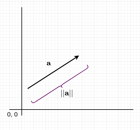
A vector is an object with path and magnitude. Take into account the velocity with which you drive a automotive. If we don’t quantify in what path the automotive goes, then it’s not a vector. But when we specify that the automotive is heading east, then it might be a vector and thus it is going to be referred to as velocity. Geometrically, it’s a line phase with an arrow pointing in a sure path. In printed texts, it may be denoted by a boldface letter resembling a or an arrow over the common letter. On this article, we are going to use boldface letters. The magnitude of a vector a is given by ∥a∥ as proven in Determine 1. On the whole, ∥a∥ can be referred to as a norm. In a 2-dimensional coordinate house, some extent is denoted by an ordered pair (x,y). Every finish of the vector could also be outlined by two such ordered pairs (x,y), and (u,v). A aircraft consisting of all such ordered pairs is known as vector house. For all actual numbers, a 2-dimensional vector house is denoted by ℝ².
Internal-products
The inside product is a option to multiply two vectors and the result’s a scalar amount (i.e., only a magnitude with no notion of a path). If two vectors are a and b denoted by ordered pair (x,y) and (u, v), then their inside product is xu* + yv* the place u* is the complicated conjugate of u and v* is the complicated conjugate of v. After all, when these numbers are actual numbers, then complicated conjugate is similar because the quantity itself. The inside product can be denoted by〈a, b〉.
Orthogonality
Two vectors a and b are orthogonal if their inside product 〈a, b〉= 0. In such a case, the projection of 1 vector onto one other collapses to a degree and we get a distance of zero. A listing of vectors is known as orthonormal if the vectors within the listing are pairwise orthogonal and every vector has a norm equal to 1.
Gram-Schmidt Orthonormalization
The Gram-Schmidt Orthonormalization process converts a listing of linearly unbiased vectors into orthonormal vectors. I’ll clarify this process with an instance.
Take into account three vectors in three-dimensional vector house: a(1, -1, 1), b(1, 0, 1), and c(1, 1, 2). The brand new listing of vectors we search is [u, v, w].
- u = a = (1, -1, 1).
- v = b – (〈b, u〉⋅ u/||u||² ) = (1/3, 2/3, 1/3)
- w = c – (〈c, u〉⋅ u/||u||² ) – (〈c, v〉⋅ v/||v||² ) = ( -1/2, 0, 1/2)
These are orthogonal vectors. Now, we normalize them to get the orthonormal vectors by dividing them by their norms, and thus we get u(√3/3, -√3/3, √3/3), v(√6/6, √6/3, √6/6), w(-√2/2, 0, √2/2).
Now, again to the enterprise.
A polynomial can be utilized in the same method as vectors, i.e., they obey an orthogonality relationship just like orthogonal vectors over a given vary [a,b]. In such a way, for a polynomial p(x), and q(x) in a variable x, we are able to outline their inside product as

the place w(x) is any non-negative perform within the vary [a,b]. Apparently, we are able to additionally carry out the Gram-Schmidt process on polynomials to get orthogonal polynomials. For example, we are able to carry out orthonormalization on [1, x, x², …] and get a household of orthogonal polynomials. We will get completely different households of polynomials relying on the selection of w(x). For instance:
- For w(x) = 1 on the interval [-1, 1], we get the Legendre polynomials.
- For w(x) = 1/sqrt(1-x²) on [-1,-1] we get the Chebyshev polynomials of the primary type.
- For w(x) = sqrt(1-x²) on [-1, 1] we get the Chebyshev polynomials of the second type.
- For w(x) = exp(-x) on [0, ∞] we get the Laguerre polynomials.
Some properties of Orthogonal Polynomials:
- If pₙ(x) is a polynomial of diploma n, then

thus, pₙ(x) is orthogonal to all polynomials of diploma lower than n-1.
2. Additional, with the selection of coefficients aₙ and bₙ relying on you select w(x), we now have the next recurrence relation:

Property no. 2 is acknowledged in Favard’s theorem, given a three-term recurrence as acknowledged above, there exists w(x), and vice-versa.
Gaussian Quadrature for Approximating Particular Integration
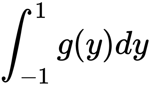
Gaussian quadrature is a technique of calculating the particular integral

We take into account a variable substitution x = ( b — a)y /2 + (a + b) y/2, and g(y) = (b-a)* f(x) /2 that converts the above particular integral to
Whereas midpoint guidelines and trapezoidal guidelines are easiest with regards to numerically evaluating the above particular integral, there exists a rule that evaluates the above integral precisely. Numerically, the above integral is written as
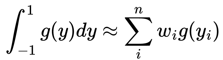
which requires an acceptable selection of yᵢ and wᵢ. On this case, Carl Friedrich Gauss devised that if we decide yᵢ to be the roots of an orthogonal polynomial pₙ(y) related to w(y), then we are able to combine the polynomial of diploma 2n-1 precisely. This rule is known as the Gauss Quadrature rule. Clearly, the only case may be when wᵢ = 1 which is the case of the Legendre polynomials. Utilizing Legendre polynomials, we get the Gauss-Legendre quadrature rule.
The Gauss quadrature is extraordinarily environment friendly as investigated by Lloyd N. Trefethen in https://epubs.siam.org/doi/abs/10.1137/060659831.
Orthogonal Polynomial Regression
Often in a linear regression mannequin strategy, selecting an acceptable order of the polynomial is critical. Within the model-building technique, we match knowledge to the mannequin in rising order and take a look at the importance of regression coefficients at every step of mannequin becoming. That is the ahead choice technique. We preserve rising the order till the t-test for the best order is non-significant.
We even have a backward elimination technique the place we begin with an acceptable highest order mannequin and begin eliminating every highest order time period till we get a big t-test statistic for the remaining highest order time period.
The ahead choice technique and the backward elimination technique don’t essentially result in the identical mannequin. Nonetheless, we could search a mannequin the place including a brand new time period of upper order merely refines the mannequin with out recalculation. This can’t be achieved by the powers of the variable x in succession. However it may be achieved by the system of orthogonal polynomials. If a linear regression has a type y = Xβ + ε then the equal orthogonal polynomial regression mannequin is given by

