Evaluating the effectiveness of coaching a number of ML fashions specialised on totally different teams, versus coaching one distinctive mannequin for all the info

I not too long ago heard an organization declaring:
“We now have 60 churn fashions in manufacturing.”
I requested them why so many. They replied that they personal 5 manufacturers working in 12 nations and, since they wished to develop one mannequin for every mixture of name and nation, that quantities to 60 fashions.
So, I requested them:
“Did you strive with simply 1 mannequin?”
They argued that it wouldn’t make sense as a result of their manufacturers are very totally different from one another, and so are the nations they function in: “You can not practice one single mannequin and anticipate it to work effectively each on an American buyer of name A and on a German buyer of name B”.
Since I’ve typically heard claims like this within the business, I used to be curious to examine if this thesis is mirrored within the information or whether it is simply hypothesis not backed up by information.
This is the reason, on this article, I’ll systematically evaluate two approaches:
- Feed all the info to a single mannequin, aka one basic mannequin;
- Construct one mannequin for every section (within the earlier instance, the mix of name and nation), aka many specialised fashions.
I’ll check these two methods on 12 actual datasets offered by Pycaret, a well-liked Python library.
How do these two approaches work, precisely?
Suppose we’ve got a dataset. The dataset consists of a matrix of predictors (known as X) and a goal variable (known as y). Furthermore, X comprises a number of columns that may very well be used to section the dataset (within the earlier instance, these columns had been “model” and “nation”).
Now let’s attempt to signify these parts graphically. We are able to use one of many columns of X to visualise the segments: every coloration (blue, yellow, and crimson) identifies a unique section. We can even want a further vector to signify the cut up in coaching set (inexperienced) and check set (pink).

Given these parts, right here is how the 2 approaches differ.
1st technique: Basic mannequin
A novel mannequin is fitted on the entire coaching set, then its efficiency is measured on the entire check set:

2nd technique: Specialised fashions
This second technique includes constructing a mannequin for every section, which implies repeating the practice/check process okay occasions (the place okay is the variety of segments, on this case 3).

Observe that, in actual use instances, the variety of segments could also be related, from a number of dozens to lots of. As a consequence, utilizing specialised fashions includes a number of sensible disadvantages in comparison with utilizing one basic mannequin, comparable to:
- increased upkeep effort;
- increased system complexity;
- increased (cumulated) coaching time;
- increased computational prices;
- increased storage prices.
So, why would anybody wish to do it?
The supporters of specialised fashions declare {that a} distinctive basic mannequin could also be much less exact on a given section (say American prospects) as a result of it has realized additionally the traits of various segments (e.g. European prospects).
I feel that is a false notion born of the utilization of easy fashions (e.g. logistic regression). Let me clarify with an instance.
Think about that we’ve got a dataset of vehicles, consisting of three columns:
- automotive kind (basic or trendy);
- automotive age;
- automotive worth.
We wish to use the primary two options to foretell the automotive worth. These are the info factors:

As you’ll be able to see, primarily based on the automotive kind, there are two fully totally different behaviors: as time passes, trendy vehicles depreciate, whereas basic vehicles improve their worth.
Now, if we practice a linear regression on the complete dataset:
linear_regression = LinearRegression().match(df[["car_type_classic", "car_age"]], df["car_price"])
The ensuing coefficients are:

This means that the mannequin will at all times predict the identical worth, 12, for any enter.
Usually, easy fashions don’t work effectively if the dataset comprises totally different behaviors (except you do extra characteristic engineering). So, on this case, one could also be tempted to coach two specialised fashions: one for traditional vehicles and one for contemporary vehicles.
However let’s see what occurs if — as a substitute of linear regression — we use a call tree. To make the comparability truthful, we are going to develop a tree with 3 splits (i.e. 3 resolution thresholds), since additionally linear regression had 3 parameters (the three coefficients).
decision_tree = DecisionTreeRegressor(max_depth=2).match(df[["car_type_classic", "car_age"]], df["car_price"])
That is the end result:

This is much better than the end result we obtained with the linear regression!
The purpose is that tree-based fashions (comparable to XGBoost, LightGBM, or Catboost) are able to coping with totally different behaviors as a result of they natively work effectively with characteristic interactions.
That is the primary purpose why there is no such thing as a theoretical purpose to favor a number of specialised fashions over one basic mannequin. However, as at all times, we don’t settle with the theoretical clarification. We additionally wish to make it possible for this conjecture is backed up by actual information.
On this paragraph, we are going to see the Python code obligatory to check which technique works higher. If you’re not within the particulars, you’ll be able to soar straight to the subsequent paragraph, the place I talk about the outcomes.
We goal to quantitatively evaluate two methods:
- coaching one basic mannequin;
- coaching many specialised fashions.
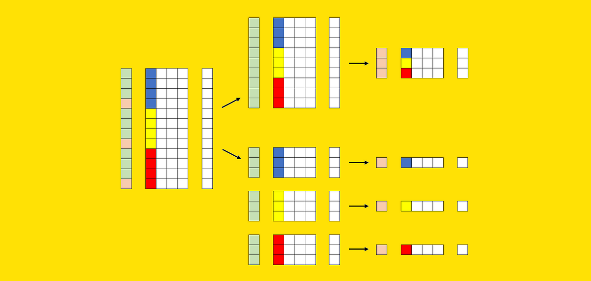
The obvious technique to evaluate them is the next:
- take a dataset;
- select a section of the dataset, primarily based on the worth of 1 column;
- cut up the dataset right into a coaching and a check dataset;
- practice a basic mannequin on the entire coaching dataset;
- practice a specialised mannequin on the portion of the coaching dataset that belongs to the section;
- evaluate the efficiency of the final mannequin and the specialised mannequin, each on the portion of the check dataset that belongs to the section.
Graphically:

This works simply superb however, since we don’t wish to get fooled by probability, we are going to repeat this course of:
- for various datasets;
- utilizing totally different columns to section the dataset itself;
- utilizing totally different values of the identical column to outline the section.
In different phrases, that is what we are going to do, in pseudocode:
for every dataset:
practice basic mannequin on the coaching set
for every column of the dataset:
for every worth of the column:
practice specialised mannequin on the portion of the coaching set for which column = worth
evaluate efficiency of basic mannequin vs. specialised mannequin
Really, we might want to make some tiny changes to this process.
To start with, we mentioned that we’re utilizing the columns of the dataset to section the dataset itself. This works effectively for categorical columns and for discrete numeric columns which have few values. For the remaining numeric columns, we should make them categorical by binning.
Secondly, we can not merely use all of the columns. If we did that, we’d be penalizing the specialised mannequin. Certainly, if we select a section primarily based on a column that has no relationship with the goal variable, there could be no purpose to consider that the specialised mannequin can carry out higher. To keep away from that, we are going to solely use the columns which have some relationship with the goal variable.
Furthermore, for the same purpose, we won’t use all of the values of the segmentation columns. We’ll keep away from values which are too frequent (extra frequent than 50%) as a result of it wouldn’t make sense to anticipate {that a} mannequin educated on nearly all of the dataset has a unique efficiency from a mannequin educated on the complete dataset. We can even keep away from values which have lower than 100 instances within the check set as a result of the end result wouldn’t be vital for certain.
In gentle of this, that is the complete code that I’ve used:
for dataset_name in tqdm(dataset_names):# get information
X, y, num_features, cat_features, n_classes = get_dataset(dataset_name)
# cut up index in coaching and check set, then practice basic mannequin on the coaching set
ix_train, ix_test = train_test_split(X.index, test_size=.25, stratify=y)
model_general = CatBoostClassifier().match(X=X.loc[ix_train,:], y=y.loc[ix_train], cat_features=cat_features, silent=True)
pred_general = pd.DataFrame(model_general.predict_proba(X.loc[ix_test, :]), index=ix_test, columns=model_general.classes_)
# create a dataframe the place all of the columns are categorical:
# numerical columns with greater than 5 distinctive values are binnized
X_cat = X.copy()
X_cat.loc[:, num_features] = X_cat.loc[:, num_features].fillna(X_cat.loc[:, num_features].median()).apply(lambda col: col if col.nunique() <= 5 else binnize(col))
# get an inventory of columns that aren't (statistically) unbiased
# from y in line with chi 2 independence check
candidate_columns = get_dependent_columns(X_cat, y)
for segmentation_column in candidate_columns:
# get an inventory of candidate values such that every candidate:
# - has no less than 100 examples within the check set
# - is just not extra widespread than 50%
vc_test = X_cat.loc[ix_test, segmentation_column].value_counts()
nu_train = y.loc[ix_train].groupby(X_cat.loc[ix_train, segmentation_column]).nunique()
nu_test = y.loc[ix_test].groupby(X_cat.loc[ix_test, segmentation_column]).nunique()
candidate_values = vc_test[(vc_test>=100) & (vc_test/len(ix_test)<.5) & (nu_train==n_classes) & (nu_test==n_classes)].index.to_list()
for worth in candidate_values:
# cut up index in coaching and check set, then practice specialised mannequin
# on the portion of the coaching set that belongs to the section
ix_value = X_cat.loc[X_cat.loc[:, segmentation_column] == worth, segmentation_column].index
ix_train_specialized = checklist(set(ix_value).intersection(ix_train))
ix_test_specialized = checklist(set(ix_value).intersection(ix_test))
model_specialized = CatBoostClassifier().match(X=X.loc[ix_train_specialized,:], y=y.loc[ix_train_specialized], cat_features=cat_features, silent=True)
pred_specialized = pd.DataFrame(model_specialized.predict_proba(X.loc[ix_test_specialized, :]), index=ix_test_specialized, columns=model_specialized.classes_)
# compute roc rating of each the final mannequin and the specialised mannequin and save them
roc_auc_score_general = get_roc_auc_score(y.loc[ix_test_specialized], pred_general.loc[ix_test_specialized, :])
roc_auc_score_specialized = get_roc_auc_score(y.loc[ix_test_specialized], pred_specialized)
outcomes = outcomes.append(pd.Sequence(information=[dataset_name, segmentation_column, value, len(ix_test_specialized), y.loc[ix_test_specialized].value_counts().to_list(), roc_auc_score_general, roc_auc_score_specialized],index=outcomes.columns),ignore_index=True)
For simpler comprehension, I’ve omitted the code of some utility capabilities, like get_dataset, get_dependent_columns and get_roc_auc_score. Nevertheless, yow will discover the complete code in this GitHub repo.
To make a large-scale comparability of basic mannequin vs. specialised fashions, I’ve used 12 real-world datasets which are obtainable in Pycaret (a Python library underneath MIT license).
For every dataset, I discovered the columns that present some vital relationship with the goal variable (p-value < 1% on the Chi-square check of independence). For any column, I’ve saved solely the values that aren’t too uncommon (they should have no less than 100 instances within the check set) or too frequent (they have to account for not more than 50% of the dataset). Every of those values identifies a section of the dataset.
For each dataset, I educated a basic mannequin (CatBoost, with no parameter tuning) on the entire coaching dataset. Then, for every section, I educated a specialised mannequin (once more CatBoost, with no parameter tuning) on the portion of the coaching dataset that belongs to the respective section. Lastly, I’ve in contrast the efficiency (space underneath the ROC curve) of the 2 approaches on the portion of the check dataset that belongs to the section.
Let’s take a glimpse on the last output:

In precept, to elect the winner, we might simply take a look at the distinction between “roc_general” and “roc_specialized”. Nevertheless, in some instances, this distinction could also be resulting from probability. So, I’ve additionally calculated when the distinction is statistically vital (see this text for particulars about how you can inform whether or not the distinction between two ROC scores is critical).
Thus, we will classify the 601 comparisons in two dimensions: whether or not the final mannequin is healthier than the specialised mannequin and whether or not this distinction is critical. That is the end result:

It’s straightforward to see that the final mannequin outperforms the specialised mannequin 89% of the time (454 + 83 out of 601). However, if we follow the numerous instances, the final mannequin outperforms the specialised mannequin 95% of the time (83 out of 87).
Out of curiosity, let’s additionally visualize the 87 vital instances in a plot, with the ROC rating of the specialised mannequin on the x-axis and the ROC rating of the final mannequin on the y-axis.

All of the factors above the diagonal establish instances wherein the final mannequin carried out higher than the specialised mannequin.
However, how higher?
We are able to compute the imply distinction between the 2 ROC scores. It seems that, within the 87 vital instances, the ROC of the final mannequin is on common 2.4% increased than the specialised mannequin, which is rather a lot!
On this article, we in contrast two methods: utilizing a basic mannequin educated on the entire dataset vs. utilizing many fashions specialised on totally different segments of the dataset.
We now have seen that there is no such thing as a compelling purpose to make use of specialised fashions since highly effective algorithms (comparable to tree-based fashions) can natively take care of totally different behaviors. Furthermore, utilizing specialised fashions includes a number of sensible issues from the perspective of upkeep effort, system complexity, coaching time, computational prices, and storage prices.
We additionally examined the 2 methods on 12 actual datasets, for a complete of 601 doable segments. On this experiment, the final mannequin outperformed the specialised mannequin 89% of the time. Wanting solely on the statistically vital instances, the quantity rises to 95%, with a median acquire of two.4% within the ROC rating.
