An intuitive rationalization
Whereas deciphering the coefficient of one of many predictors (say a steady variable X1) of an empirical mannequin — with a number of explanatory variables (X1, X2, …..Xn) predicting the worth of an end result variable (Y) — you have to have used these statements: “controlling for different elements/holding different elements fixed/accounting for different elements/holding different elements mounted, one unit improve in X1 is, on common, related to b items improve in Y.” However what precisely does it imply to manage for a variable/maintain a variable fixed/account for a variable/maintain a variable fixed? As a newbie in information science, I actually struggled to know these questions:
- What does it imply to manage for a variable?
- How precisely will we management for a variable?
- Why will we even want to manage for a variable?
Looking back, I feel the confusion originated as a result of I believed regression is about becoming a straight line by some dots (which is right however there are different methods of conceptualizing regression). On this article, utilizing an intuitive toy instance, I’ll attempt to clarify these three questions. I’m deliberately utilizing MS Excel for this text. Though as an information analyst I choose different choices, I consider Excel is a superior device for explicitly displaying what’s inside a black field to a wider inhabitants.
We match/estimate empirical fashions utilizing linear regression for 2 functions:
- Predicting the worth of an end result (for instance, annual gross sales of a retailer)
- Estimating the causal impact of a specific therapy/motion/ intervention on an end result (for instance, the impact of accepting a consumer’s card on the month-to-month spending of shoppers at a retailer).
I’ll come again to the dialogue on predictive modeling later. For now, let’s concentrate on the second cause for estimating an empirical mannequin utilizing regression.
Final month, a grocery chain XYZ provided a consumer’s card to all the shoppers who visited its shops within the metropolis of ABC. A few of the prospects accepted the cardboard, others didn’t. The chain has shops in 10 different cities, and earlier than introducing the cardboard in different cities, they’re attempting to know how efficient accepting the consumer’s card was when it comes to affecting the month-to-month spending of those that accepted it. You’ve got been employed because the analyst to analyze the query!
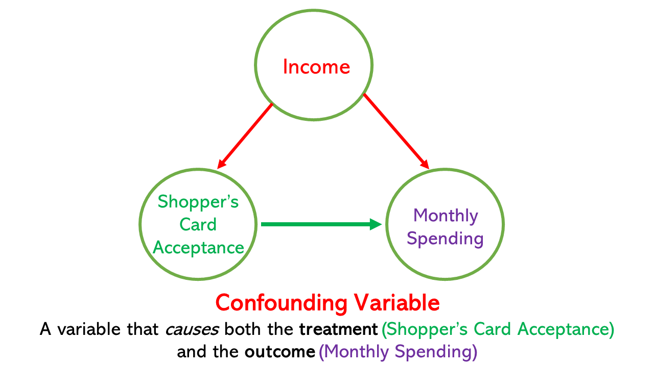
To begin with, you understand that the shopper’s card was neither randomly provided nor randomly accepted. As you may have been skilled in causal modeling, you might be frightened about confounding variables, i.e., elements that have an effect on each the therapy (accepting the consumer’s card) and have an effect on the end result (month-to-month spending on the retailer).
You do some background research on the traits of those that accepted the cardboard and people who didn’t. After cautious exploration, you determine that revenue is the one distinction between the 2 teams. Greater-income prospects had been extra prone to settle for the consumer’s card; furthermore, based mostly in your prior information, you realize that higher-income prospects usually tend to spend extra on the retailer. You might be assured in making the belief that aside from revenue, the 2 teams are, on common, an identical.
Earlier than you estimate the mannequin utilizing a regression, you draw the next directed acyclic graph (DAG) to explicitly showcase your key assumption:
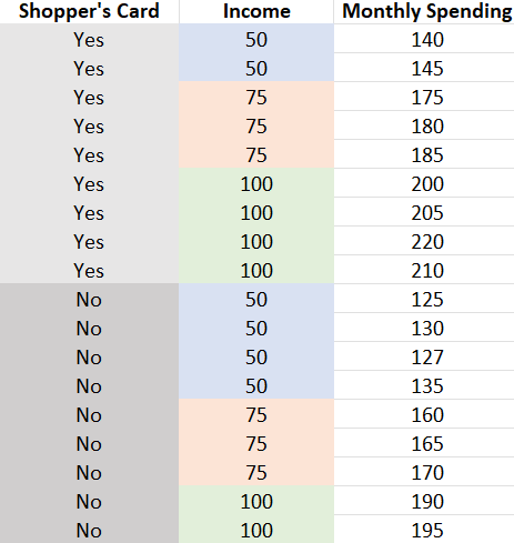
Now, let’s have a look at the dataset. For simplicity, let’s faux, there are solely three revenue teams: $50k, $75k, and $100k.
As a result of revenue is the one confounding variable (Shopper’s Card Acceptance ← Revenue → Month-to-month Spending), we’ve got to “management for” revenue to estimate the causal impact of accepting the consumer’s card on month-to-month spending. However why? 🤔
Controlling for revenue means evaluating the month-to-month spending of the 2 teams (i.e., prospects who accepted the cardboard and prospects who didn’t settle for the cardboard) inside a specific revenue class.
As you assumed, the one distinction between the 2 teams is revenue. Given this assumption is right:
- When you examine those that accepted the cardboard and people who didn’t inside a sure revenue class then it’s as if the 2 teams are apples-to-apples (or as if randomly assigned).
- Due to this fact, the 2 teams are an identical apart from one group accepted the cardboard whereas the opposite didn’t.
- Lastly, inside a sure revenue class, if there’s a distinction in month-to-month spending, you’ll be able to attribute that distinction to the consumer’s card acceptance.
One other manner to consider that is that controlling for revenue closes the backdoor path Shopper’s Card Acceptance ← Revenue → Month-to-month Spending, and so, the affiliation from Shopper’s Card Acceptance to Month-to-month Spending can stream solely by the true causal path Shopper’s Card Acceptance → Month-to-month Spending.
Now, let’s calculate the income-category-specific distinction in spending between these with and with out a shopper’s card:

Right here, inside the $50k revenue group, the distinction in spending between the 2 teams is $13.25. Equally, the distinction inside the $75k group is $15, and the $100k group is $16.25. These three are income-group-specific common causal results. Did you discover that we held/saved the worth of revenue fixed in every of the three instances? 😊
Nonetheless, your boss needs a particular quantity, and never three separate numbers. So, you might want to work out a option to weight these three numbers into one estimate. You weight every income-category-specific causal estimate by the proportion of individuals (in your complete pattern) current in that particular revenue group. On this easy instance, we’ve got a complete of 18 prospects and there are 6 prospects in every of the three revenue classes. So, all three estimates get a weight of 6/18 = 1/3 every. Lastly, you get the next:
Common Causal Impact= 13.25*(1/3) + 15*(1/3) + 16.25*(1/3) = 14.83
At this level, you could be pondering that this can be a lot of labor! 😓 Additionally, we don’t get a regular error of the Common Causal Impact by this guide method. 😔
That is precisely why relatively than calculating the above manually, you’ll choose estimating the next mannequin utilizing linear regression:
Month-to-month Spending = b0 + b1*Shopper’s Card Acceptance + b2*Income50 +b3*Income75+ e
the place Shopper’s Card Acceptance is a dummy variable that takes a worth of 1 if a buyer accepts the cardboard and a 0 in any other case; Income50 is a dummy which takes a worth of 1 if a buyer has $50k revenue; Income75 is a dummy which takes a worth of 1 if a buyer has $75k revenue. And, e is the error time period which consists of all different causes of Month-to-month Spending; importantly, none of those different causes has any impact on whether or not a buyer accepts a consumer’s card **since you assumed it solely is dependent upon Revenue which you already accounted for within the mannequin.**
Once I match the above mannequin, that is the regression output:
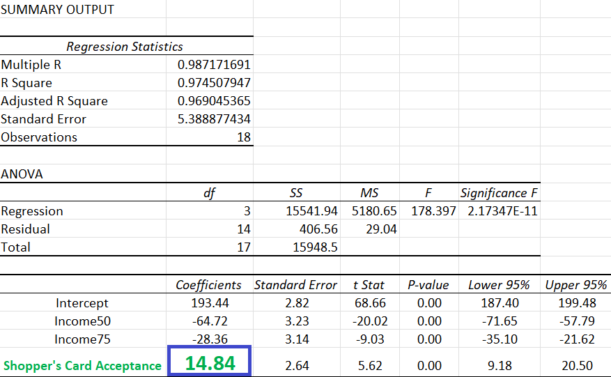
Environment friendly and beautiful! Isn’t it? 🥰 With the a number of regression method, we will management for Revenue and get the Common Causal Impact of accepting a consumer’s card on the month-to-month spending conduct with commonplace error, t-stat, p-value, and a 95% confidence interval!
Additionally, should you don’t consider within the causal assumption talked about earlier (i.e., revenue is the one confounder), you’ll be able to interpret the coefficient of the Shopper’s Card Acceptance variable as: “Controlling for Revenue, individuals who accepted shopper’s card, on common, spent $14.84 extra per thirty days on the retailer in comparison with individuals who didn’t settle for shopper’s card.”
**You’ll have seen there’s a slight distinction between the regression estimated impact (14.84) and the true impact (14.83). It’s because regression gives a “bizarre” variance-weighted causal impact (and never the proper weighted one we estimated manually). I created this pretend dataset in a manner that the deviation is negligible. Within the subsequent article, I’ll elaborate on this concern.**
Now let’s take into consideration one other state of affairs. You’ve got been tasked with predicting the annual gross sales of retailer XYZ for the subsequent 10 years. On this case, the interpretation of every predictor’s coefficient is meaningless. All you care about is the predictive success of your mannequin. You’ll be able to actually throw the kitchen sink at your mannequin. Add all the flamboyant quadratic and interplay phrases. Most significantly, you care about any statistic that reveals you ways nicely the mannequin matches the info (e.g. R², adjusted R², AIC, and many others.). I’ve seen folks deciphering the coefficients of predictive fashions. I’m sorry — it simply doesn’t make any sense to me. 🙇Why? Take into consideration the next state of affairs (I defined it intimately in one other article).
You are attempting to foretell the worth of the variety of folks attacked by sharks on a sea seaside and also you got here up with the next mannequin:
Month-to-month Shark Assaults = -2.02+0.03*Month-to-month Ice Cream Gross sales
This mannequin matches the info fairly nicely! If you realize the ice cream gross sales in a specific month, you’ll be able to predict the worth of shark assaults in that month with affordable precision. However what’s the purpose in deciphering the coefficient of the predictor? 🤦Sure, you could say “one unit improve in month-to-month ice cream gross sales is, on common, related to a 0.03 unit improve in month-to-month shark assaults.” When you had one other predictor Z, you’ll have added “Controlling for Z” firstly of the earlier assertion. However once more, why trouble deciphering? Are you able to counsel that “the constructive affiliation suggests if ice cream gross sales are curtailed/banned, many lives may very well be saved from shark assaults”? That will be nonsensical!😒
I’ll finish this text by summarizing the important thing factors I mentioned above.
Once we examine the causal impact of a therapy/motion/intervention with non-experimental information, we have to “management for” confounding variables.
Controlling for a variable means estimating the distinction in end result between the therapy group and the management group inside a particular class/worth of the managed variable.
Regression is a handy estimation technique that helps us management for confounding variables.
There’s completely no level in deciphering the coefficients of the predictors of a predictive mannequin (whether or not you management for different variables or not).
