
Learn to create an LSTM-based neural community to foretell an univariate time collection

On this article you’ll learn to make a prediction from a time collection with Tensorflow and Keras in Python.
We’ll use a sequential neural community created in Tensorflow based mostly on bidirectional LSTM layers to seize the patterns within the univariate sequences that we are going to enter to the mannequin.
Specifically we’ll see how
- generate artificial information to simulate a time collection with totally different traits
- course of the information in coaching and validation units and create a dataset based mostly on time home windows
- outline an structure for our neural community utilizing LSTM (lengthy short-term reminiscence)
- prepare and consider the mannequin
The purpose of this tutorial is to foretell some extent sooner or later given a sequence of knowledge. The multi-step case won’t be lined, the place the earlier level is predicted which has in flip been predicted by the mannequin.
This information is impressed on Coursera’s DeepLearning.AI TensorFlow Developer specialization, which I extremely counsel any reader to take a look at.
Let’s start.
As an alternative of downloading a dataset from the net, we’ll use features that may permit us to generate an artificial time collection for our case. We will even use dataclasses to retailer our time collection parameters in a category in order that we are able to use them no matter scope. The dataclass identify will likely be G, which stands for “international”.
I made a decision to make use of this strategy as a substitute of utilizing an actual dataset as a result of this methodology permits us to check a number of time collection and have flexibility within the inventive technique of our tasks.
Let’s generate an artificial time collection with this code
That is the obtained collection

Now that now we have a usable time collection, let’s transfer on to preprocessing.
The peculiarity of the time collection is that they should be divided into coaching and validation units and which in flip should be divided into sequences of a size outlined by our configuration. These sequences are known as home windows and the mannequin will use these sequences to provide a forecast.
Let’s see two extra helper features to realize this.
Right here some explanations are due. The train_val_split operate merely divides our collection based mostly on the G.SPLIT_TIME worth beforehand outlined within the G dataclass. Moreover, we’ll cross it the G.TIME and G.SERIES parameters.
Let’s recall the definition of the G dataclass.

By calling generate_time_series, we receive
TIME = vary(0, 1439)
SERIES = array([ 0.81884814, 0.82252744, 0.77998762, …, -0.44389692, -0.42693424, -0.39230758])
Each of size 1439.
The break up of train_val_split will likely be equal to
time_train = vary(0, 1100)
time_val = vary(1100, 1439)
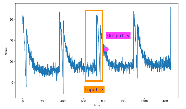
After dividing into coaching and validation units we’ll use some Tensorflow features to create a Dataset object that may permit us to create the X options and the y goal. Recall that X are the n values that the mannequin will use to foretell the subsequent, which might be y.
Let’s see easy methods to implement these features
We’ll use Tensorflow’s .window() methodology on the dataset object to use a shift of 1 to our factors. An instance of the utilized logic might be seen right here:

Within the instance we create a variety from 0 to 10 with Tensorflow, and apply a window of 5. We’ll then create a complete of 5 columns. Passing shift = 1 every column could have one much less worth ranging from the highest and drop_remainder = True will be sure that you at all times have a matrix of the identical measurement.
Let’s apply these two features.
Now that the information is prepared we are able to transfer on to structuring our neural community.
As talked about originally of the article, our neural community will primarily be based mostly on LSTM (long-short time period reminiscence) layers. What makes an LSTM appropriate for this sort of job is that it has an inside construction able to propagating data by way of lengthy sequences.
This makes them very helpful in pure language processing (NLP) and exactly in time collection, as a result of these two forms of duties might require the switch of data throughout all the sequence.
Within the following code we’ll see how the LSTM layers are included inside a Bidirectional layer. This layer permits the LSTM to contemplate the sequence of knowledge in each instructions and subsequently to have context not solely of the previous but in addition of the longer term. It can assist us construct a community that will likely be extra exact than a one-way one.
Along with LSTMs, there are additionally GRUs (Gated Recurrent Models) that can be utilized for time collection prediction duties.
We will even use the Lambda layer which is able to permit us to accurately adapt the enter information format to our community and eventually a dense layer to calculate the ultimate output.
Let’s see easy methods to implement all this in Keras and Tensorflow sequentially.
The Lambda layer permits us to make use of customized features inside a layer. We use it to be sure that the dimensionality of the enter is enough for the LSTM. Since our dataset consists of two-dimensional time home windows, the place the primary is the batch_size and the opposite is timesteps.
Nevertheless, an LSTM accepts a 3rd dimension, which signifies the variety of dimensions of our enter. Through the use of the Lambda operate and input_shape = [None], we’re successfully telling Tensorflow to simply accept any sort of enter dimension. That is useful as a result of we don’t have to put in writing further code to make sure the dimensionality is right.
To learn extra about LSTM and the way the layer works, I invite the reader to seek the advice of the official Tensorflow information current right here.
All LSTM layers are included inside a Bidirectional layer, and every of them passes the processed sequences to the subsequent layer by way of return_sequences = True.
If this argument have been False, Tensorflow would give an error, for the reason that subsequent LSTM wouldn’t discover a sequence from to course of. The one layer that should not return the sequences is the final LSTM, for the reason that last dense layer is the one liable for offering the ultimate prediction and never one other sequence.
As you may learn within the article Management the coaching of your neural community in Tensorflow with callbacks, we’ll use a callback to cease the coaching when our efficiency metric reaches a specified stage. We’ll use the imply absolute error (MAE) to measure how nicely our community is ready to accurately predict the subsequent level within the collection.
In reality, this can be a comparable job to a regression job, and subsequently will use comparable efficiency metrics.
Let’s see the code to implement early stopping.
We’re prepared to coach our LSTM mannequin. We outline a operate that may name create_uncompiled_model and can present the mannequin with a loss operate and an optimizer.
The Huber loss operate can be utilized to steadiness between the imply absolute error, or MAE, and the imply sq. error, MSE. It’s subsequently a very good loss operate for when you’ve gotten numerous information or just a few outliers, as on this case.
The Adam optimizer is a usually legitimate selection — let’s set an arbitrary learning_rate of 0.001.
Let’s begin the coaching

We see that on the twentieth epoch the goal MAE is reached and the coaching is stopped.
Let’s plot the curves for the loss and the MAE.

The curves present an enchancment of the web till it stabilizes after the fifth epoch. It’s nonetheless a very good end result.
Let’s write a helper operate for straightforward entry to MAE and MSE. As well as, we additionally outline a operate to create predictions.
Let’s see now how the mannequin performs! Let’s make predictions on the entire collection and on the validation set.
Let’s see the outcomes on the validation set

And on all the collection

The outcomes seem like good. Maybe now we have a approach to improve the mannequin’s efficiency by rising the coaching durations or by enjoying with the educational price.
mse: 30.91, mae: 3.32 forecast.
Let’s see now easy methods to predict some extent sooner or later given the final sequence within the collection.
And right here’s the end result (amended — the picture reveals 200 factors).

In abstract, now we have seen easy methods to
- generate an artificial time collection
- divide the collection into X and y appropriately
- construction a neural community in Keras and Tensorflow based mostly on bidirectional LSTMs
- prepare with early stopping and consider efficiency
- make predictions in regards to the coaching collection, validation and into the longer term
In case you have any ideas on easy methods to enhance this circulate, write within the feedback and share your methodology. I hope the article may also help you together with your tasks.
Keep nicely 👋
