
An ARMA or autoregressive shifting common mannequin is a forecasting mannequin that predicts future values based mostly on previous values. Forecasting is a vital job for a number of enterprise goals, resembling predictive analytics, predictive upkeep, product planning, budgeting, and many others. An enormous benefit of ARMA fashions is that they’re comparatively easy. They solely require a small dataset to make a prediction, they’re extremely correct for brief forecasts, they usually work on knowledge with out a pattern.
On this tutorial, we’ll learn to use the Python statsmodels bundle to forecast knowledge utilizing an ARMA mannequin and InfluxDB, the open supply time collection database. The tutorial will define use the InfluxDB Python shopper library to question knowledge from InfluxDB and convert the information to a Pandas DataFrame to make working with the time collection knowledge simpler. Then we’ll make our forecast.
I’ll additionally dive into some great benefits of ARMA in additional element.
Necessities
This tutorial was executed on a macOS system with Python 3 put in by way of Homebrew. I like to recommend establishing further tooling like virtualenv, pyenv, or conda-env to simplify Python and shopper installations. In any other case, the total necessities are right here:
- influxdb-client = 1.30.0
- pandas = 1.4.3
- influxdb-client >= 1.30.0
- pandas >= 1.4.3
- matplotlib >= 3.5.2
- sklearn >= 1.1.1
This tutorial additionally assumes that you’ve a free tier InfluxDB cloud account and that you’ve created a bucket and created a token. You’ll be able to consider a bucket as a database or the best hierarchical stage of knowledge group inside InfluxDB. For this tutorial we’ll create a bucket referred to as NOAA.
What’s ARMA?
ARMA stands for auto-regressive shifting common. It’s a forecasting approach that may be a mixture of AR (auto-regressive) fashions and MA (shifting common) fashions. An AR forecast is a linear additive mannequin. The forecasts are the sum of previous values occasions a scaling issue plus the residuals. To study extra concerning the math behind AR fashions, I counsel studying this text.
A shifting common mannequin is a collection of averages. There are various kinds of shifting averages together with easy, cumulative, and weighted varieties. ARMA fashions mix the AR and MA strategies to generate a forecast. I like to recommend studying this submit to study extra about AR, MA, and ARMA fashions. At the moment we’ll be utilizing the statsmodels ARMA operate to make forecasts.
Assumptions of AR, MA, and ARMA fashions
Should you’re trying to make use of AR, MA, and ARMA fashions then you could first guarantee that your knowledge meets the necessities of the fashions: stationarity. To judge whether or not or not your time collection knowledge is stationary, you could verify that the imply and covariance stay fixed. Fortunately we are able to use InfluxDB and the Flux language to acquire a dataset and make our knowledge stationary.
We’ll do that knowledge preparation within the subsequent part.
Flux for time collection differencing and knowledge preparation
Flux is the information scripting language for InfluxDB. For our forecast, we’re utilizing the Air Sensor pattern dataset that comes out of the field with InfluxDB. This dataset accommodates temperature knowledge from a number of sensors. We’re making a temperature forecast for a single sensor. The information appears like this:
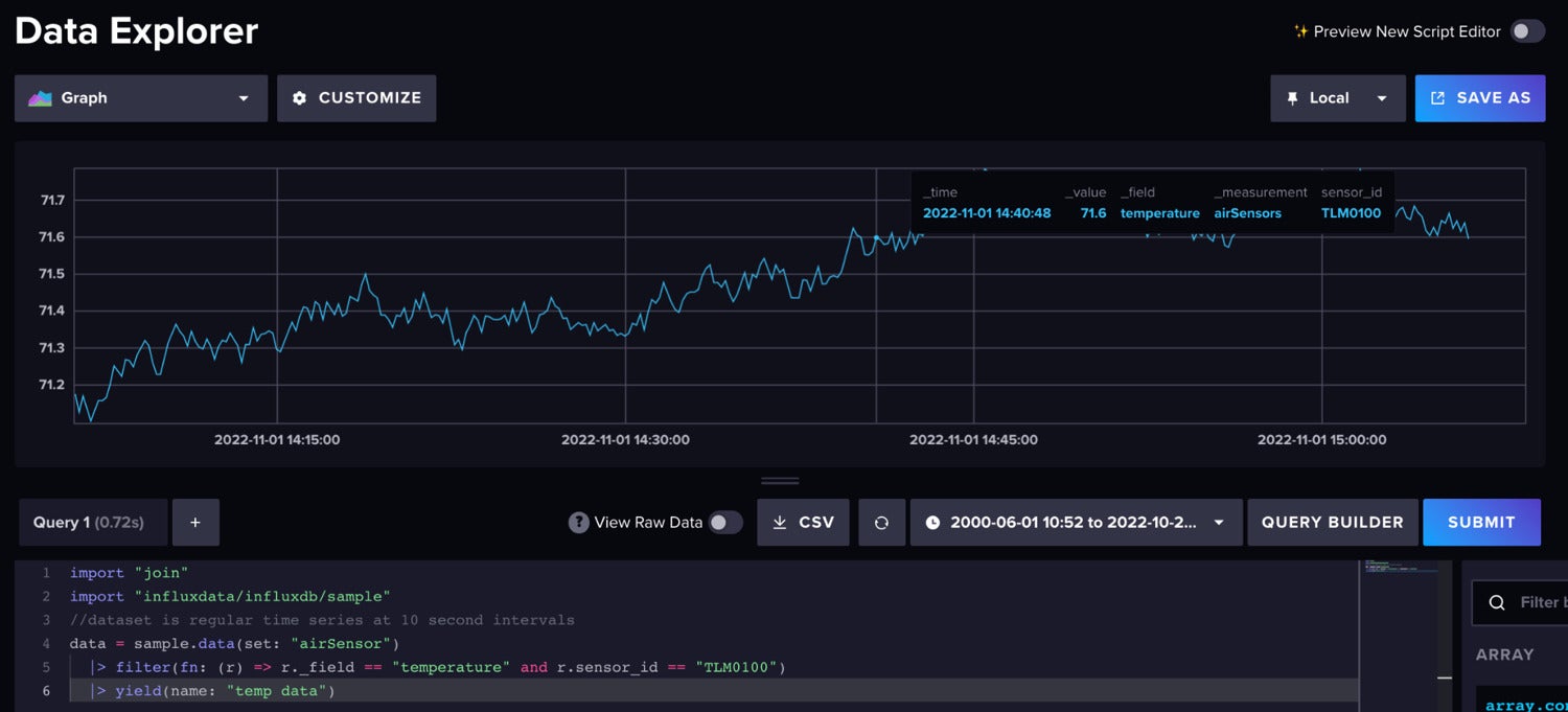 InfluxData
Use the next Flux code to import the dataset and filter for the one time collection.
import "be a part of"
import "influxdata/influxdb/pattern"
//dataset is common time collection at 10 second intervals
knowledge = pattern.knowledge(set: "airSensor")
  |> filter(fn: (r) => r._field == "temperature" and r.sensor_id == "TLM0100")
Subsequent we are able to make our time collection weakly stationary by differencing the shifting common. Differencing is a method to take away any pattern or slope from our knowledge. We’ll use shifting common differencing for this knowledge preparation step. First we discover the shifting common of our knowledge.
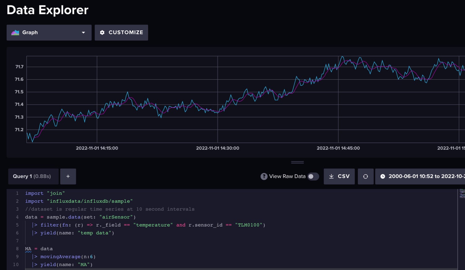 InfluxData
Uncooked air temperature knowledge (blue) vs. the shifting common (pink).
Subsequent we subtract the shifting common from our precise time collection after becoming a member of the uncooked knowledge and MA knowledge collectively.
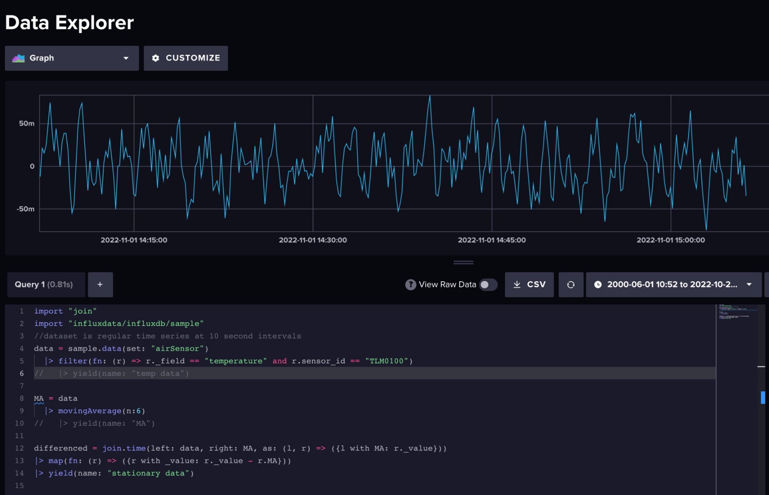 InfluxData
The differenced knowledge is stationary.
Right here is your complete Flux script used to carry out this differencing:
import "be a part of"
import "influxdata/influxdb/pattern"
//dataset is common time collection at 10 second intervals
knowledge = pattern.knowledge(set: "airSensor")
  |> filter(fn: (r) => r._field == "temperature" and r.sensor_id == "TLM0100")
//   |> yield(identify: "temp knowledge")

MA = knowledge
  |> movingAverage(n:6)
//   |> yield(identify: "MA")

differenced = be a part of.time(left: knowledge, proper: MA, as: (l, r) => ({l with MA: r._value}))
|> map(fn: (r) => ({r with _value: r._value - r.MA}))
|> yield(identify: "stationary knowledge")
Please word that this strategy estimates the pattern cycle. Sequence decomposition is commonly carried out with linear regression as effectively.
ARMA and time collection forecasts with Python
Now that we’ve ready our knowledge, we are able to create a forecast. We should determine the p worth and q worth of our knowledge so as to use the ARMA methodology. The p worth defines the order of our AR mannequin. The q worth defines the order of the MA mannequin. To transform the statsmodels ARIMA operate to an ARMA operate we offer a d worth of 0. The d worth is the variety of nonseasonal variations wanted for stationarity. Since we don’t have seasonality we don’t want any differencing.
First we question our knowledge with the Python InfluxDB shopper library. Subsequent we convert the DataFrame to an array. Then we match our mannequin, and at last we make a prediction.
# question knowledge with the Python InfluxDB Shopper Library and take away the pattern by way of differencing
shopper = InfluxDBClient(url="https://us-west-2-1.aws.cloud2.influxdata.com", token="NyP-HzFGkObUBI4Wwg6Rbd-_SdrTMtZzbFK921VkMQWp3bv_e9BhpBi6fCBr_0-6i0ev32_XWZcmkDPsearTWA==", org="0437f6d51b579000")
# write_api = shopper.write_api(write_options=SYNCHRONOUS)
query_api = shopper.query_api()
df = query_api.query_data_frame('import "be a part of"'
'import "influxdata/influxdb/pattern"'
'knowledge = pattern.knowledge(set: "airSensor")'
  '|> filter(fn: (r) => r._field == "temperature" and r.sensor_id == "TLM0100")'
'MA = knowledge'
  '|> movingAverage(n:6)'
'be a part of.time(left: knowledge, proper: MA, as: (l, r) => ({l with MA: r._value}))'
'|> map(fn: (r) => ({r with _value: r._value - r.MA}))'
'|> maintain(columns:["_value", "_time"])'
'|> yield(identify:"differenced")'
)
df = df.drop(columns=['table', 'result'])
y = df["_value"].to_numpy()
date = df["_time"].dt.tz_localize(None).to_numpy()
y = pd.Sequence(y, index=date)
mannequin = sm.tsa.arima.ARIMA(y, order=(1,0,2))
end result = mannequin.match()
Ljung-Field take a look at and Durbin-Watson take a look at
The Ljung-Field take a look at can be utilized to confirm that the values you used for p,q for becoming an ARMA mannequin are good. The take a look at examines autocorrelations of the residuals. Primarily it assessments the null speculation that the residuals are independently distributed. When utilizing this take a look at, your aim is to verify the null speculation or present that the residuals are in truth independently distributed. First you could suit your mannequin with chosen p and q values, like we did above. Then use the Ljung-Field take a look at to find out if these chosen values are acceptable. The take a look at returns a Ljung-Field p-value. If this p-value is larger than 0.05, then you’ve gotten efficiently confirmed the null speculation and your chosen values are good.
After becoming the mannequin and operating the take a look at with Python…
print(sm.stats.acorr_ljungbox(res.resid, lags=[5], return_df=True))
we get a p-value for the take a look at of 0.589648.
| lb_stat | lb_pvalue |
|---|---|
| 5 3.725002 | 0.589648 |
This confirms that our p,q values are acceptable throughout mannequin becoming.
You may as well use the Durbin-Watson take a look at to check for autocorrelation. Whereas the Ljung-Field assessments for autocorrelation with any lag, the Durbin-Watson take a look at makes use of solely a lag equal to 1. The results of your Durbin-Watson take a look at can range from 0 to 4 the place a price near 2 signifies no autocorrelation. Purpose for a price near 2.
print(sm.stats.durbin_watson(end result.resid.values))
Right here we get the next worth, which agrees with the earlier take a look at and confirms that our mannequin is nice.
2.0011309357716414
Full ARMA forecasting script with Python and Flux
Now that we perceive the elements of the script, let’s have a look at the script in its entirety and create a plot of our forecast.
import pandas as pd
import numpy as np
import matplotlib.pyplot as plt
from influxdb_client import InfluxDBClient
from datetime import datetime as dt
import statsmodels.api as sm
from statsmodels.tsa.arima.mannequin import ARIMA
# question knowledge with the Python InfluxDB Shopper Library and take away the pattern by way of differencing
shopper = InfluxDBClient(url="https://us-west-2-1.aws.cloud2.influxdata.com", token="NyP-HzFGkObUBI4Wwg6Rbd-_SdrTMtZzbFK921VkMQWp3bv_e9BhpBi6fCBr_0-6i0ev32_XWZcmkDPsearTWA==", org="0437f6d51b579000")
# write_api = shopper.write_api(write_options=SYNCHRONOUS)
query_api = shopper.query_api()
df = query_api.query_data_frame('import "be a part of"'
'import "influxdata/influxdb/pattern"'
'knowledge = pattern.knowledge(set: "airSensor")'
  '|> filter(fn: (r) => r._field == "temperature" and r.sensor_id == "TLM0100")'
'MA = knowledge'
  '|> movingAverage(n:6)'
'be a part of.time(left: knowledge, proper: MA, as: (l, r) => ({l with MA: r._value}))'
'|> map(fn: (r) => ({r with _value: r._value - r.MA}))'
'|> maintain(columns:["_value", "_time"])'
'|> yield(identify:"differenced")'
)
df = df.drop(columns=['table', 'result'])
y = df["_value"].to_numpy()
date = df["_time"].dt.tz_localize(None).to_numpy()
y = pd.Sequence(y, index=date)
mannequin = sm.tsa.arima.ARIMA(y, order=(1,0,2))
end result = mannequin.match()
fig, ax = plt.subplots(figsize=(10, 8))
fig = plot_predict(end result, ax=ax)
legend = ax.legend(loc="higher left")
print(sm.stats.durbin_watson(end result.resid.values))
print(sm.stats.acorr_ljungbox(end result.resid, lags=[5], return_df=True))
plt.present()
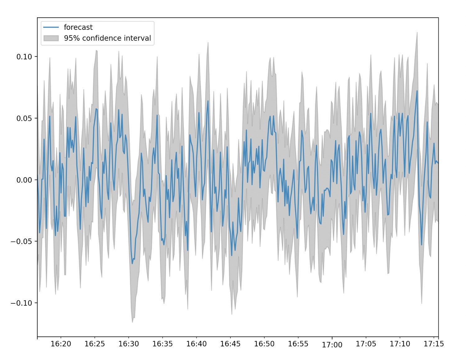 InfluxData
The underside line
I hope this weblog submit conjures up you to make the most of ARMA and InfluxDB to make forecasts. I encourage you to check out the following repo, which incorporates examples for work with each the algorithms described right here and InfluxDB to make forecasts and carry out anomaly detection.
Anais Dotis-Georgiou is a developer advocate for InfluxData with a ardour for making knowledge lovely with the usage of knowledge analytics, AI, and machine studying. She applies a mixture of analysis, exploration, and engineering to translate the information she collects into one thing helpful, priceless, and exquisite. When she just isn’t behind a display screen, you’ll find her outdoors drawing, stretching, boarding, or chasing after a soccer ball.
—
New Tech Discussion board offers a venue to discover and talk about rising enterprise know-how in unprecedented depth and breadth. The choice is subjective, based mostly on our decide of the applied sciences we imagine to be essential and of best curiosity to InfoWorld readers. InfoWorld doesn’t settle for advertising and marketing collateral for publication and reserves the fitting to edit all contributed content material. Ship all inquiries to newtechforum@infoworld.com.
Copyright © 2022 IDG Communications, Inc.
