
This put up is a tutorial on how one can use TensorFlow Estimators for textual content classification.
Be aware: This put up was written along with the superior Julian Eisenschlos and was initially revealed on the TensorFlow weblog.
Hiya there! All through this put up we are going to present you how one can classify textual content utilizing Estimators in TensorFlow. Right here’s the define of what we’ll cowl:
- Loading information utilizing Datasets.
- Constructing baselines utilizing pre-canned estimators.
- Utilizing phrase embeddings.
- Constructing customized estimators with convolution and LSTM layers.
- Loading pre-trained phrase vectors.
- Evaluating and evaluating fashions utilizing TensorBoard.
Welcome to Half 4 of a weblog sequence that introduces TensorFlow Datasets and Estimators. You don’t must learn the entire earlier materials, however have a look if you wish to refresh any of the next ideas. Half 1 targeted on pre-made Estimators, Half 2 mentioned function columns, and Half 3 how one can create customized Estimators.
Right here in Half 4, we are going to construct on high of all of the above to deal with a special household of issues in Pure Language Processing (NLP). Specifically, this text demonstrates how one can resolve a textual content classification process utilizing customized TensorFlow estimators, embeddings, and the tf.layers module. Alongside the way in which, we’ll study word2vec and switch studying as a method to bootstrap mannequin efficiency when labeled information is a scarce useful resource.
We’ll present you related code snippets. Right here’s the entire Jupyter Pocket book you can run domestically or on Google Colaboratory. The plain .py supply file can be accessible right here. Be aware that the code was written to reveal how Estimators work functionally and was not optimized for optimum efficiency.
The duty
The dataset we will probably be utilizing is the IMDB Giant Film Overview Dataset, which consists of extremely polar film critiques for coaching, and for testing. We’ll use this dataset to coach a binary classification mannequin, capable of predict whether or not a evaluate is constructive or unfavourable.
For illustration, right here’s a chunk of a unfavourable evaluate (with stars) within the dataset:
Now, I LOVE Italian horror movies. The cheesier they’re, the higher. Nevertheless, this isn’t tacky Italian. That is week-old spaghetti sauce with rotting meatballs. It’s novice hour on each stage. There isn’t a suspense, no horror, with just some drops of blood scattered round to remind you that you’re the truth is watching a horror movie.
Keras supplies a handy handler for importing the dataset which can be accessible as a serialized numpy array .npz file to obtain right here. For textual content classification, it’s customary to restrict the dimensions of the vocabulary to stop the dataset from turning into too sparse and excessive dimensional, inflicting potential overfitting. Because of this, every evaluate consists of a sequence of phrase indexes that go from (essentially the most frequent phrase within the dataset the) to , which corresponds to orange. Index represents the start of the sentence and the index is assigned to all unknown (also referred to as out-of-vocabulary or OOV) tokens. These indexes have been obtained by pre-processing the textual content information in a pipeline that cleans, normalizes and tokenizes every sentence first after which builds a dictionary indexing every of the tokens by frequency.
After we’ve loaded the information in reminiscence we pad every of the sentences with $0$ in order that we now have two $25000 occasions 200$ arrays for coaching and testing respectively.
vocab_size = 5000
sentence_size = 200
(x_train_variable, y_train), (x_test_variable, y_test) = imdb.load_data(num_words=vocab_size)
x_train = sequence.pad_sequences(
    x_train_variable,
    maxlen=sentence_size,
    padding='put up',
    worth=0)
x_test = sequence.pad_sequences(
    x_test_variable,
    maxlen=sentence_size,
    padding='put up',
    worth=0)
Enter Capabilities
The Estimator framework makes use of enter capabilities to separate the information pipeline from the mannequin itself. A number of helper strategies can be found to create them, whether or not your information is in a .csv file, or in a pandas.DataFrame, whether or not it matches in reminiscence or not. In our case, we will use Dataset.from_tensor_slices for each the prepare and take a look at units.
x_len_train = np.array([min(len(x), sentence_size) for x in x_train_variable])
x_len_test = np.array([min(len(x), sentence_size) for x in x_test_variable])

def parser(x, size, y):
    options = {"x": x, "len": size}
    return options, y

def train_input_fn():
    dataset = tf.information.Dataset.from_tensor_slices((x_train, x_len_train, y_train))
    dataset = dataset.shuffle(buffer_size=len(x_train_variable))
    dataset = dataset.batch(100)
    dataset = dataset.map(parser)
    dataset = dataset.repeat()
    iterator = dataset.make_one_shot_iterator()
    return iterator.get_next()

def eval_input_fn():
    dataset = tf.information.Dataset.from_tensor_slices((x_test, x_len_test, y_test))
    dataset = dataset.batch(100)
    dataset = dataset.map(parser)
    iterator = dataset.make_one_shot_iterator()
    return iterator.get_next()
We shuffle the coaching information and don’t predefine the variety of epochs we wish to prepare, whereas we solely want one epoch of the take a look at information for analysis. We additionally add an extra "len" key that captures the size of the unique, unpadded sequence, which we are going to use later.
Constructing a baseline
It’s good apply to begin any machine studying venture attempting primary baselines. The easier the higher as having a easy and sturdy baseline is vital to understanding precisely how a lot we’re gaining by way of efficiency by including additional complexity. It might very properly be the case {that a} easy answer is nice sufficient for our necessities.
With that in thoughts, allow us to begin by attempting out one of many easiest fashions for textual content classification. That may be a sparse linear mannequin that offers a weight to every token and provides up the entire outcomes, whatever the order. As this mannequin doesn’t care concerning the order of phrases in a sentence, we usually seek advice from it as a Bag-of-Phrases method. Let’s see how we will implement this mannequin utilizing an Estimator.
We begin out by defining the function column that’s used as enter to our classifier. As we now have seen in Half 2, categorical_column_with_identity is the best alternative for this pre-processed textual content enter. If we have been feeding uncooked textual content tokens different feature_columns may do numerous the pre-processing for us. We are able to now use the pre-made LinearClassifier.
column = tf.feature_column.categorical_column_with_identity('x', vocab_size)
classifier = tf.estimator.LinearClassifier(
    feature_columns=[column],
    model_dir=os.path.be part of(model_dir, 'bow_sparse'))
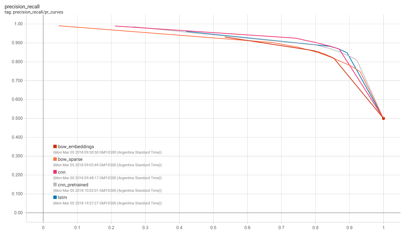
Lastly, we create a easy perform that trains the classifier and moreover creates a precision-recall curve. As we don’t goal to maximise efficiency on this weblog put up, we solely prepare our fashions for 25,000 steps.
def train_and_evaluate(classifier):
    classifier.prepare(input_fn=train_input_fn, steps=25000)
    eval_results = classifier.consider(input_fn=eval_input_fn)
    predictions = np.array([p['logistic'][0] for p in classifier.predict(input_fn=eval_input_fn)])
    tf.reset_default_graph()
    # Add a PR abstract along with the summaries that the classifier writes
    pr = summary_lib.pr_curve('precision_recall', predictions=predictions, labels=y_test.astype(bool), num_thresholds=21)
    with tf.Session() as sess:
        author = tf.abstract.FileWriter(os.path.be part of(classifier.model_dir, 'eval'), sess.graph)
        author.add_summary(sess.run(pr), global_step=0)
        author.shut()
train_and_evaluate(classifier)
One of many advantages of selecting a easy mannequin is that it’s way more interpretable. The extra complicated a mannequin, the tougher it’s to examine and the extra it tends to work like a black field. On this instance, we will load the weights from our mannequin’s final checkpoint and try what tokens correspond to the greatest weights in absolute worth. The outcomes seem like what we might anticipate.
weights = classifier.get_variable_value('linear/linear_model/x/weights').flatten()

extremes = np.concatenate((sorted_indexes[-8:], sorted_indexes[:8]))

extreme_weights = sorted(
    [(weights[i], word_inverted_index[i - index_offset]) for i in extremes])

y_pos = np.arange(len(extreme_weights))
plt.bar(y_pos, [pair[0] for pair in extreme_weights], align='heart', alpha=0.5)
plt.xticks(y_pos, [pair[1] for pair in extreme_weights], rotation=45, ha='proper')
plt.ylabel('Weight')
plt.title('Most important tokens')
plt.present()
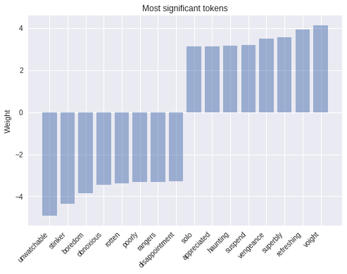
As we will see, tokens with essentially the most constructive weight corresponding to ‘refreshing’ are clearly related to constructive sentiment, whereas tokens which have a big unfavourable weight unarguably evoke unfavourable feelings. A easy however highly effective modification that one can do to enhance this mannequin is weighting the tokens by their tf-idf scores.
Embeddings
The subsequent step of complexity we will add are phrase embeddings. Embeddings are a dense low-dimensional illustration of sparse high-dimensional information. This permits our mannequin to study a extra significant illustration of every token, quite than simply an index. Whereas a person dimension will not be significant, the low-dimensional area—when discovered from a big sufficient corpus—has been proven to seize relations corresponding to tense, plural, gender, thematic relatedness, and lots of extra. We are able to add phrase embeddings by changing our current function column into an embedding_column. The illustration seen by the mannequin is the imply of the embeddings for every token (see the combiner argument within the docs). We are able to plug within the embedded options right into a pre-canned DNNClassifier.
A be aware for the eager observer: an embedding_column is simply an environment friendly means of making use of a completely linked layer to the sparse binary function vector of tokens, which is multiplied by a relentless relying of the chosen combiner. A direct consequence of that is that it wouldn’t make sense to make use of an embedding_column immediately in a LinearClassifier as a result of two consecutive linear layers with out non-linearities in between add no prediction energy to the mannequin, until after all the embeddings are pre-trained.
embedding_size = 50
word_embedding_column = tf.feature_column.embedding_column(
    column, dimension=embedding_size)
classifier = tf.estimator.DNNClassifier(
    hidden_units=[100],
    feature_columns=[word_embedding_column],
    model_dir=os.path.be part of(model_dir, 'bow_embeddings'))
train_and_evaluate(classifier)
We are able to use TensorBoard to visualise our $50$ dimensional phrase vectors projected into $mathbb{R}^3$ utilizing t-SNE. We anticipate comparable phrases to be shut to one another. This is usually a helpful method to examine our mannequin weights and discover sudden behaviours.
Convolutions
At this level one attainable method can be to go deeper, additional including extra absolutely linked layers and taking part in round with layer sizes and coaching capabilities. Nevertheless, by doing that we might add additional complexity and ignore vital construction in our sentences. Phrases don’t reside in a vacuum and that means is compositional, shaped by phrases and its neighbors.
Convolutions are one method to benefit from this construction, much like how we will mannequin salient clusters of pixels for picture classification. The instinct is that sure sequences of phrases, or n-grams, normally have the identical that means no matter their general place within the sentence. Introducing a structural prior through the convolution operation permits us to mannequin the interplay between neighboring phrases and consequently offers us a greater method to symbolize such that means.
The next picture exhibits how a filter matrix $F in mathbb{R}^{dtimes m}$ tri-gram window of tokens to construct a brand new function map. Afterwards a pooling layer is normally utilized to mix adjoining outcomes.
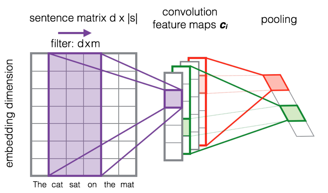
Supply: Studying to Rank Quick Textual content Pairs with Convolutional Deep Neural Networks by Severyn et al. [2015]
Allow us to have a look at the total mannequin structure. Using dropout layers is a regularization approach that makes the mannequin much less prone to overfit.
Making a customized estimator
As seen in earlier weblog posts, the tf.estimator framework supplies a high-level API for coaching machine studying fashions, defining prepare(), consider() and predict() operations, dealing with checkpointing, loading, initializing, serving, constructing the graph and the session out of the field. There’s a small household of pre-made estimators, like those we used earlier, but it surely’s more than likely that you will want to construct your individual.
Writing a customized estimator means writing a model_fn(options, labels, mode, params) that returns an EstimatorSpec. Step one will probably be mapping the options into our embedding layer:
input_layer = tf.contrib.layers.embed_sequence(
    options['x'],
    vocab_size,
    embedding_size,
    initializer=params['embedding_initializer'])
Then we use tf.layers to course of every output sequentially.
coaching = (mode == tf.estimator.ModeKeys.TRAIN)
dropout_emb = tf.layers.dropout(inputs=input_layer,
                                charge=0.2,
                                coaching=coaching)
conv = tf.layers.conv1d(
    inputs=dropout_emb,
    filters=32,
    kernel_size=3,
    padding="similar",
    activation=tf.nn.relu)
pool = tf.reduce_max(input_tensor=conv, axis=1)
hidden = tf.layers.dense(inputs=pool, models=250, activation=tf.nn.relu)
dropout = tf.layers.dropout(inputs=hidden, charge=0.2, coaching=coaching)
logits = tf.layers.dense(inputs=dropout_hidden, models=1)
Lastly, we are going to use a Head to simplify the writing of our final a part of the model_fn. The pinnacle already is aware of how one can compute predictions, loss, train_op, metrics and export outputs, and might be reused throughout fashions. That is additionally used within the pre-made estimators and supplies us with the good thing about a uniform analysis perform throughout all of our fashions. We’ll use binary_classification_head, which is a head for single label binary classification that makes use of sigmoid_cross_entropy_with_logits because the loss perform below the hood.
head = tf.contrib.estimator.binary_classification_head()
optimizer = tf.prepare.AdamOptimizer()
def _train_op_fn(loss):
    tf.abstract.scalar('loss', loss)
    return optimizer.reduce(
        loss=loss,
        global_step=tf.prepare.get_global_step())

return head.create_estimator_spec(
    options=options,
    labels=labels,
    mode=mode,
    logits=logits,
    train_op_fn=_train_op_fn)
Operating this mannequin is simply as straightforward as earlier than:
initializer = tf.random_uniform([vocab_size, embedding_size], -1.0, 1.0))
params = {'embedding_initializer': initializer}
cnn_classifier = tf.estimator.Estimator(model_fn=model_fn,
                                        model_dir=os.path.be part of(model_dir, 'cnn'),
                                        params=params)
train_and_evaluate(cnn_classifier)
LSTM Networks
Utilizing the Estimator API and the identical mannequin head, we will additionally create a classifier that makes use of a Lengthy Quick-Time period Reminiscence (LSTM) cell as a substitute of convolutions. Recurrent fashions corresponding to this are among the most profitable constructing blocks for NLP purposes. An LSTM processes the whole doc sequentially, recursing over the sequence with its cell whereas storing the present state of the sequence in its reminiscence.
One of many drawbacks of recurrent fashions in comparison with CNNs is that, due to the character of recursion, fashions end up deeper and extra complicated, which normally produces slower coaching time and worse convergence. LSTMs (and RNNs basically) can endure convergence points like vanishing or exploding gradients, that stated, with adequate tuning they’ll receive state-of-the-art outcomes for a lot of issues. As a rule of thumb CNNs are good at function extraction, whereas RNNs excel at duties that rely upon the that means of the entire sentence, like query answering or machine translation.
Every cell processes one token embedding at a time updating its inside state primarily based on a differentiable computation that is dependent upon each the embedding vector $x_t$ and the earlier state $h_{t-1}$. With a purpose to get a greater understanding of how LSTMs work, you possibly can seek advice from Chris Olah’s weblog put up.

Supply: Understanding LSTM Networks by Chris Olah
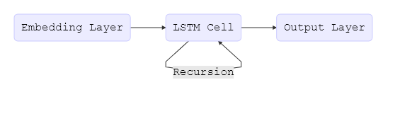
The whole LSTM mannequin might be expressed by the next easy flowchart:
To start with of this put up, we padded all paperwork as much as tokens, which is important to construct a correct tensor. Nevertheless, when a doc accommodates fewer than phrases, we don’t need the LSTM to proceed processing padding tokens because it doesn’t add info and degrades efficiency. Because of this, we moreover wish to present our community with the size of the unique sequence earlier than it was padded. Internally, the mannequin then copies the final state via to the sequence’s finish. We are able to do that by utilizing the "len" function in our enter capabilities. We are able to now use the identical logic as above and easily substitute the convolutional, pooling, and flatten layers with our LSTM cell.
lstm_cell = tf.nn.rnn_cell.BasicLSTMCell(100)
_, final_states = tf.nn.dynamic_rnn(
        lstm_cell, inputs, sequence_length=options['len'], dtype=tf.float32)
logits = tf.layers.dense(inputs=final_states.h, models=1)
Pre-trained vectors
A lot of the fashions that we now have proven earlier than depend on phrase embeddings as a primary layer. To date, we now have initialized this embedding layer randomly. Nevertheless, a lot earlier work has proven that utilizing embeddings pre-trained on a big unlabeled corpus as initialization is helpful, notably when coaching on solely a small variety of labeled examples. The most well-liked pre-trained embedding is word2vec. Leveraging information from unlabeled information through pre-trained embeddings is an occasion of switch studying.
To this finish, we are going to present you how one can use them in an Estimator. We’ll use the pre-trained vectors from one other well-liked mannequin, GloVe.
embeddings = {}
with open('glove.6B.50d.txt', 'r', encoding='utf-8') as f:
    for line in f:
        values = line.strip().cut up()
        w = values[0]
        vectors = np.asarray(values[1:], dtype='float32')
        embeddings[w] = vectors
After loading the vectors into reminiscence from a file we retailer them as a numpy.array utilizing the identical indexes as our vocabulary. The created array is of form (5000, 50). At each row index, it accommodates the 50-dimensional vector representing the phrase on the similar index in our vocabulary.
embedding_matrix = np.random.uniform(-1, 1, measurement=(vocab_size, embedding_size))
for w, i in word_index.objects():
    v = embeddings.get(w)
    if v is not None and i < vocab_size:
        embedding_matrix[i] = v
Lastly, we will use a customized initializer perform and cross it within the params object to our cnn_model_fn , with none modifications.
def my_initializer(form=None, dtype=tf.float32, partition_info=None):
    assert dtype is tf.float32
    return embedding_matrix
params = {'embedding_initializer': my_initializer}
cnn_pretrained_classifier = tf.estimator.Estimator(
    model_fn=cnn_model_fn,
    model_dir=os.path.be part of(model_dir, 'cnn_pretrained'),
    params=params)
train_and_evaluate(cnn_pretrained_classifier)
Operating TensorBoard
Now we will launch TensorBoard and see how the totally different fashions we’ve educated evaluate towards one another by way of coaching time and efficiency.
In a terminal, we run
> tensorboard --logdir={model_dir}
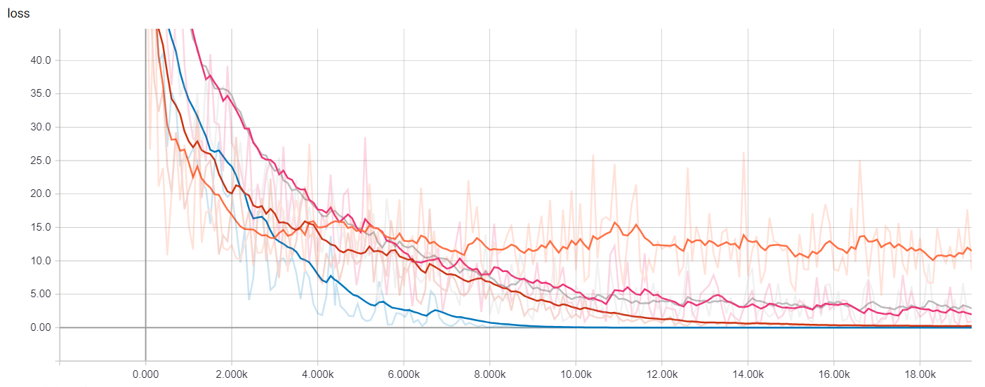
We are able to visualize many metrics collected whereas coaching and testing, together with the loss perform values of every mannequin at every coaching step, and the precision-recall curves. That is after all most helpful to pick out which mannequin works greatest for our use-case in addition to how to decide on classification thresholds.
Getting Predictions
To acquire predictions on new sentences we will use the predict technique within the Estimator situations, which is able to load the most recent checkpoint for every mannequin and consider on the unseen examples. However earlier than passing the information into the mannequin we now have to wash up, tokenize and map every token to the corresponding index as we see under.
def text_to_index(sentence):

    translator = str.maketrans('', '', string.punctuation.substitute("'", ''))
    tokens = sentence.translate(translator).decrease().cut up()
    return np.array([1] + [word_index[t] + index_offset if t in word_index else 2 for t in tokens])

def print_predictions(sentences, classifier):
    indexes = [text_to_index(sentence) for sentence in sentences]
    x = sequence.pad_sequences(indexes,
                               maxlen=sentence_size,
                               padding='put up',
                               worth=-1)
    size = np.array([min(len(x), sentence_size) for x in indexes])
    predict_input_fn = tf.estimator.inputs.numpy_input_fn(x={"x": x, "len": size}, shuffle=False)
    predictions = [p['logistic'][0] for p in classifier.predict(input_fn=predict_input_fn)]
    print(predictions)
It’s price noting that the checkpoint itself will not be adequate to make predictions; the precise code used to construct the estimator is important as properly so as to map the saved weights to the corresponding tensors. It’s apply to affiliate saved checkpoints with the department of code with which they have been created.
In case you are desirous about exporting the fashions to disk in a completely recoverable means, you may wish to look into the SavedModel class, which is particularly helpful for serving your mannequin via an API utilizing TensorFlow Serving.
Abstract
On this weblog put up, we explored how one can use estimators for textual content classification, specifically for the IMDB Opinions Dataset. We educated and visualized our personal embeddings, in addition to loaded pre-trained ones. We began from a easy baseline and made our method to convolutional neural networks and LSTMs.
For extra particulars, you should definitely try:
Thanks for studying!
