Statistics Bootcamp 7: Balancing Kind I and II Errors | by Adrienne Kline | Nov, 2022

Be taught the maths and strategies behind the libraries you employ every day as an information scientist

This text is an element of a bigger Bootcamp sequence (see kicker for full listing!). This one is devoted to understanding Kind 1 and a pair of errors and introducing the t-distribution.

Any choice we make primarily based on speculation testing could also be incorrect. We are able to reject once we ought to have accepted, and vice versa. This arises once we use a single pattern to tell chances in regards to the inhabitants as an entire.

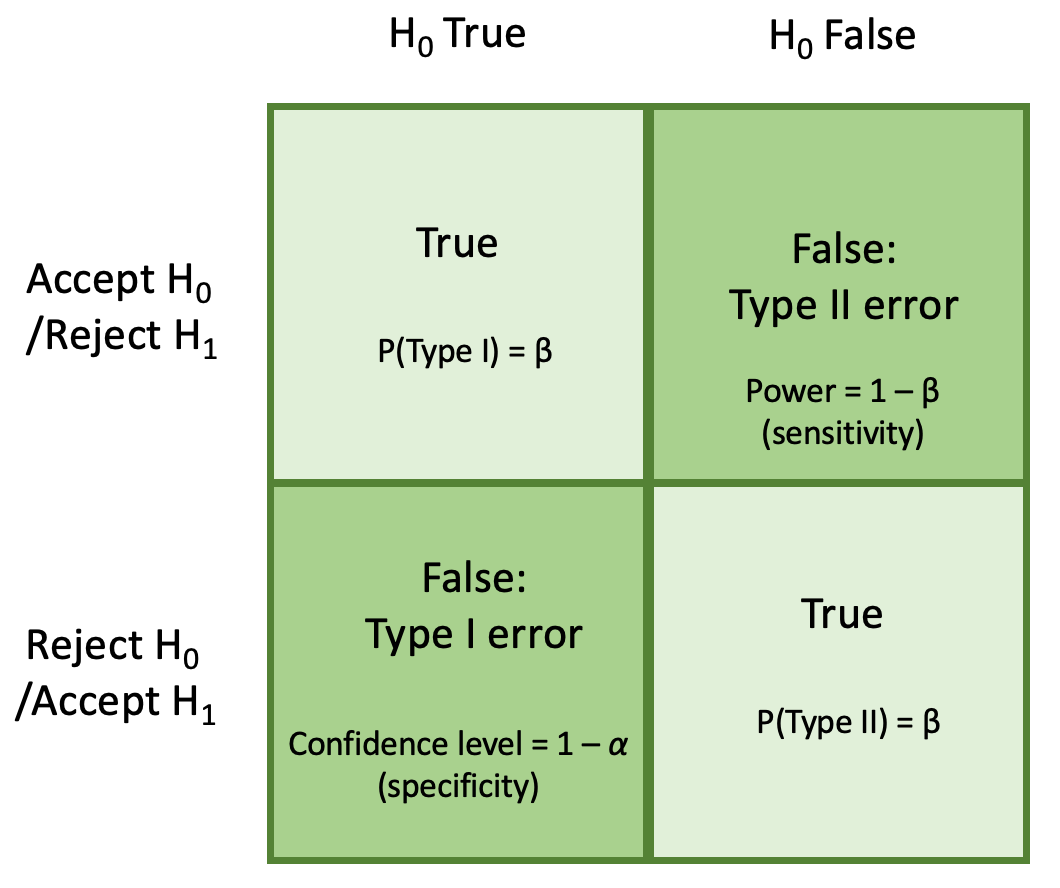
In statistics, we take into account two forms of errors, relying on the directionality of floor fact of the scenario (which we not often know) however can estimate. There are Kind I and Kind II errors. A Kind I error is when we’ve got rejected the null speculation once we shouldn’t have, i.e. the null speculation = true. Conversely, a Kind II error has occurred when we’ve got didn’t reject the null speculation (accepted the null speculation), once we shouldn’t have, i.e. the null speculation = False. You may see the contingency desk beneath for a visible illustration of this phenomenon.

Graphically, we are able to symbolize this as:

Instance.
H₀: μ = 150 lbs (the common feminine weighs 150 lbs)
H₁: μ ≠ 150 lbs (the common feminine doesn’t weigh 150 lbs)

A sort I error has occurred if the bottom fact is μ = 150 lbs, however the knowledge evaluation has led to the conclusion that μ ≠ 150 lbs. Conversely, a sort II error has occurred if the bottom fact is μ ≠ 150 lbs, however the knowledge evaluation has led to the conclusion that μ = 150 lbs.

Now, each kind I and kind II errors have a sure chance of occurring. The chance, P of a Kind I error, is denoted P(Kind I error) = α, and we confer with this as our significance stage in statistics. That is the chance of rejecting the null speculation by sheer probability and is the world beneath the curve (AUC).
P(Kind I error) = P(reject H₀ | H₀ is true)

The chance, P of a Kind II error, is denoted P(Kind II error) = β. That is the chance of not rejecting the null speculation when it’s false and the choice speculation is true.
P(Kind II error) = P(fail to reject H₀ | H₁ is true)
or:
P(Kind II error) = P(fail to reject H₀ | H₀ is fake)

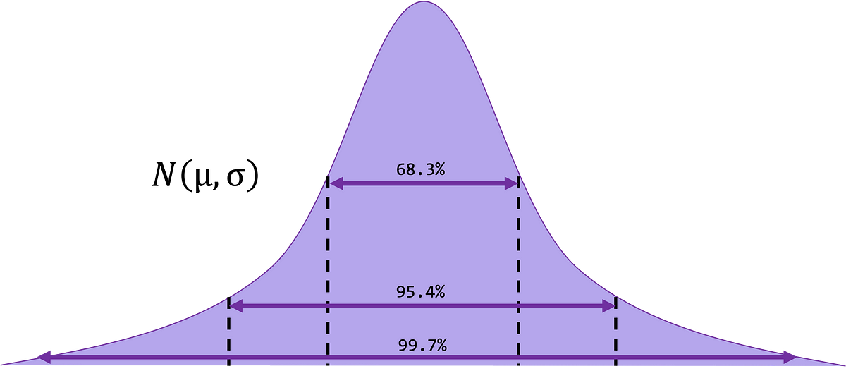
We have now to steadiness the chance of α in opposition to the chance of β, as these two commerce off. As a result of the smaller α is, the bigger the worth of β is and vice versa, assuming pattern dimension is stored fixed. We are able to see that represented visually right here:

If we take into consideration sliding these distributions over each other, if we lower α (Kind I error) by shifting the proper distribution farther proper, we inevitably enhance the worth of β (Kind II error).

Coming again to our contingency desk from above, we are able to fill what we’ve got discovered and the way we are able to incorporate it into what we discovered beforehand.

A chance worth (P-value) refers back to the space beneath the distribution curve that denotes the chance of getting the end result we observe (take a look at statistic) from our knowledge if the null speculation is true. This tells us how ‘stunned’ we must be by our outcomes — i.e. how a lot proof we’ve got in opposition to H₀ and in favor of H₁. As earlier than, we’ve got 3 totally different sorts of checks: two-tailed, right-tailed and left-tailed.

Observe that for the two-tailed take a look at, we’ve got to multiply our P-value by 2, so we’ve got the identical chance (5%, if α = 0.05) at both tail in any other case it defaults to 1/2 of what we’d need — 0.025 or 2.5%. It ought to come as no shock that in case your P-value could be very small (that means it’s location is on the far tail(s) of the distribution) that it turns into extra seemingly that H₀ is fake as there may be extra proof to recommend that it’s the farther away from the imply of the distribution.

In our final bootcamp, we discovered speculation testing with the z-statistic primarily based on the crucial worth method, the place we comply with the identical first 4 steps outlined beneath when fixing utilizing the p-value method. The place we differ is step 5. As an alternative of figuring out our crucial factors, we’ll decide the corresponding p-values to the calculated statistic.

One Pattern z-test (P-value method)

We at the moment are going to debate speculation testing utilizing a p-value method. Our assumptions are the identical as earlier: easy random pattern, regular and/or giant inhabitants, σ is understood.s

1. State our null and various hypotheses — H₀ (μ = μ) and H₁.
2. Decide from our hypotheses if this constitutes a proper (μ > μ₀), left (μ < μ₀) or two-tailed take a look at (μ ≠ μ₀).
3. Confirm our significance stage α.
4. Compute the take a look at statistic primarily based on our knowledge

5. Decide our p-value (space beneath distribution) primarily based on the take a look at statistic from our corresponding z-table.

6. Examine our P-value to α.

7. Make the choice to reject or not reject the null speculation. If P-value ≤ α, reject the null speculation. If P-value > α, don’t reject the null speculation.

8. Interpret your findings — ‘there may be ample proof to assist the rejection of the null’ OR ‘there may be not ample proof to reject the null speculation’.

In case you are questioning whether or not these 2 strategies (crucial v. p-value) give totally different outcomes — they don’t. They’re simply two other ways to consider the identical phenomenon. With the crucial worth method, you’re evaluating your statistic to the crucial worth immediately. Within the p-value method, you’re evaluating the related space beneath the curve (AUC) related to that very same crucial worth and take a look at statistic.

Instance (p-value method). A librarian needs to see if the imply variety of books her college students take a look at each day is >50. She collects a pattern over books checked out for 30 random weekdays in the course of the scool 12 months that are foudn to havea imply of 52 books. At α = 0.05, take a look at the declare that the imply quantity books take a look at is >50/college day. The usual deviation of the imply is 4 books.

Let’s verify our assumptions: 1) we’ve got obtained a random pattern, 2) pattern dimension is n=30, which is ≥ 30, 3) the usual deviation (σ) of the inhabitants is understood.

1. State the hypotheses. H₀: μ = 50, H₁: μ > 50
2. Directionality of the take a look at: right-tailed take a look at (since we’re testing ‘better than’)
3. Our significance stage is α = 0.05
4. Compute the take a look at statistic worth.

5. Decide our p-value (space beneath distribution) primarily based on the take a look at statistic from our corresponding z-table (proper tailed). We learn the z-table by discovering 2.7 on the rows after which 0.04 within the columns to get 2.74 and the world to the left of zcalc is 0.99693, subsequently the world to the proper is 0.00361.

6. Our p-value < α = 0.05, subsequently we reject the null speculation.

7. Interpret our findings. There may be sufficient proof to assist the declare that the imply variety of books checked out in a day is >50.

Instance (p-value method). The Nature household of scientific journal that the studies the common time to assessment is 8 weeks. To see if the common price of particular person journal is totally different, a researcher selects a random pattern of 35 papers which have a median time to assessment of 9 weeks. The usual deviation (σ) is 1 week. At α = 0.01, can or not it’s concluded that the common time to assessment is totally different than 8 weeks?

Let’s verify our assumptions: 1) we’ve got obtained a random pattern, 2) pattern is 35, which is ≥ 30, 3) the usual deviation of the inhabitants is supplied.

1. State the hypotheses. H₀: μ = 8, H₁: μ ≠ 8
2. Directionality of the take a look at: two-tailed
3. α = 0.01
4. Compute the z-test statistic

5. Decide our p-value (space beneath distribution) primarily based on the take a look at statistic from our corresponding z-table (two tailed). We learn the z-table by discovering 0.1 on the rows after which 0.06 within the columns to get 0.16 and the world to the left of zcalc is 0.4364 , however we have to multiply by 2 since it is a two tailed take a look at so we get: 2(0.4364) = 0.8692.

6. Since p-value ≮ α on both aspect, it doesn’t falls into the rejection area, we reject fail to reject H₀.

7. Interpret our findings. There may be inadequate proof to assist the declare that the common time to assessment is totally different than 8 weeks.

Confidence Intervals When σ is Unknown

In prior boot camps, the examples we’ve labored by have had the inhabitants commonplace deviation, σ, supplied. Nevertheless, it’s not often recognized. To compensate when σ is unknown, we use a t-distribution and values somewhat than the usual regular N(0,1) distribution and z-score and values. The equations look very comparable. Although the ‘search for’ desk they correspond to is totally different:

Briefly, if σ (inhabitants commonplace deviation) is understood, use the z-distribution. In any other case, use the t-distribution working with ‘s’, the pattern distribution.

The t-distribution is parameterized by the levels of freedom (DOF), which will be any unsigned integer, and the worth of α. Observe that DOF is normally approximated as n (variety of samples)-1. There are a number of properties of the t-distribution:

• form is decided by DOF = n-1
• Can tackle any worth between (-inf, inf)
• it’s symmetric round 0, however flatter than our commonplace regular curve — N(0,1)

Because the DOF of a t-distribution will increase, it approaches the usual regular distribution — N(0,1). The notation for the t-distribution is denoted:

Plotting totally different t-distributions with totally different DOF we get (code beneath):

from scipy.stats import t
import matplotlib.pyplot as plt
import seaborn as sns
import numpy as np
#generate t distribution with pattern dimension 1000
x = t.rvs(df=12, dimension=1000)
y = t.rvs(df=2, dimension=1000)
z = t.rvs(df=8, dimension=1000)
#sns.kdeplot(x) # plotting t, a individually 
fig = sns.kdeplot(x, coloration="r")
fig = sns.kdeplot(y, coloration="b")
fig = sns.kdeplot(z, coloration="y")
plt.legend(loc='higher proper', labels=['df = 12', 'df = 2', 'df = 8'])
plt.present()

For a curve with 15 levels of freedom, what’s the crucial worth of t for t(0.05) in a proper tail take a look at? To seek out this, use a t-table.

One Pattern t-Interval

Now that you’re comfy figuring out t-value from t-tables, we are able to translate this into figuring out confidence interval (CI) for a given μ when σ in uknown.

Once more, our assumptions are that we’ve got obtained a easy random pattern and that pattern constitutes a standard inhabitants or is giant sufficient to imagine normality, and σ is uknown. Similar to how we calculated CIs in a z-distribution:

1. Decide the boldness stage: 1 – α
2. Decide DOF = n – 1 (the place n is pattern dimension)
3. Reference a t-table to search out t-values for t_{α/2}
4. Compute the imply and commonplace deviation of the pattern, x_bar and s respectively
5. The arrogance interval is represented as:

6. Summarize CI. ‘We are able to say that the imply of the pattern will fall inside these bounds (confidence stage) quantity of the time’.

Instance. Confidence Interval in t-test. A diabetes examine recruited 25 individuals to analyze the impact of a brand new diabetes drug program on a1c ranges. After 1 month, the themes’ a1c have been recorded beneath. Use the info to search out the 95% confidence interval for the imply lower in hemoglobin a1c, μ. Assume the pattern comes from a usually distributed inhabitants.

6.1  5.9  7.0  6.5  6.4 
5.3  7.1  6.3  5.5  7.0
7.6  6.3  6.6  7.2  5.7
6.0  5.4  5.8  6.2  6.4
5.9  6.2  6.6  6.8  7.1 

1. Our confidence stage as specified within the query is 0.95, with α = 0.05
2. DOF = n–1 = 25–1 = 24
3. The worth as per the t-table equivalent to t(24, 0.05) is:

4. The imply x_bar = 6.356 and commonplace deviation s is = 0.60213509

5. Utilizing our formulation:

6. Our interpretation of this CI is that 95% of the time the imply a1c on this inhabitants is someplace between 6.12 and 6.61

t-Take a look at: P-value vs. Crucial Worth

As indicated earlier on this article when describing the distinction between z-test approaches (crucial worth vs. p-value) the identical holds true for the t-test. They’re simply two other ways to consider the identical phenomenon. With the crucial worth method, you’re evaluating your statistic to the crucial worth immediately. Within the p-value method, you’re evaluating the related space beneath the curve (AUC) related to that very same crucial worth and take a look at statistic. The one distinction is {that a} t-test is utilized to a pattern somewhat than a inhabitants, so we calculate our levels of freedom (DOF) when discovering our values/areas. Let’s work the identical drawback implementing each answer varieties.

Instance. One Pattern t-test crucial worth method
A swimming coach claims that male swimmers are on common taller than than their feminine counterparts. A pattern of 15 male swimmers has a imply top of 188 cm with a normal deviation of 5cm. If the common top of the feminine swimmers is 175 cm, is there sufficient sufficient proof to assist this declare at α = 0.05? Asume the inhabitants is often distributed.

Let’s first verify our assumptions:

• We have now obtained a random pattern
• Inhabitants is often distributed
• The inhabitants commonplace deviation is supplied within the immediate

1. State the hypotheses. H₀: μ = 175 cm, H₁: μ > 175 cm
2. Directionality of the take a look at: right-tailed
3. α = 0.05, df = 15–1 = 14
4. Compute t(calc):

5. Discover the crucial worth, primarily based on the t-table. Since α = 0.05 and the take a look at is a right-tailed take a look at, the crucial worth is Tcrit(0.05) = 1.761. Reject H₀ if Tcalc > 1.761.

6. Since 10.07 > 1.761, it falls into the rejection area, we reject H₀.

7. Interpret our findings. There may be ample proof to assist the declare that the common male swimmers is taller than their feminine counterparts.

Instance. One Pattern t-test p-value worth method

Let’s work by the identical drawback above, however utilizing a p-value method.

1. The corresponding p-value (space beneath distribution) primarily based on the t statistic (10.07) is < .00001.
2. Since tcrit < α, it falls into the rejection area, we reject H₀.
3. Interpret our findings. There may be ample proof to assist the declare that the common male swimmers is taller than their feminine counterparts.

On this bootcamp we’ve coated errors, z versus t testing and methods to carry out statistical calculations utilizing the two principal approaches (p-value and demanding worth). After studying this text, you must perceive how altering the speed of a Kind I error influecne the speed of a Kind II error. As an FYI, Kind I errors are thought of to be extra aggregious. The rationale for that is that establishment (Ho) is our default assumption, and is healthier to default and assume no impact than declare a false one.

All photos until in any other case said are created by the creator.