Study the mathematics and strategies behind the libraries you utilize day by day as an information scientist

To extra formally deal with the necessity for a statistics lecture sequence on Medium, I’ve began to create a sequence of statistics boot camps, as seen within the title above. These will construct on each other and as such shall be numbered accordingly. The motivation for doing so is to democratize the data of statistics in a floor up trend to deal with the necessity for extra formal statistics coaching within the knowledge science group. These will start easy and broaden upwards and outwards, with workout routines and labored examples alongside the best way. My private philosophy relating to engineering, coding, and statistics is that should you perceive the mathematics and the strategies, the abstraction now seen utilizing a large number of libraries falls away and permits you to be a producer, not solely a shopper of data. Many sides of those shall be a overview for some learners/readers, nevertheless having a complete understanding and a useful resource to consult with is vital. Blissful studying/studying!
This text is devoted to introducing the conventional distribution and properties of it.
Medical researchers have decided so-called regular intervals for an individual’s blood stress, ldl cholesterol, and triglycerides.
Ex. systolic blood stress: 110–140 (these metrics differ for in workplace versus house blood stress measurements)
However our query stays, how does one decide the so-called regular intervals?
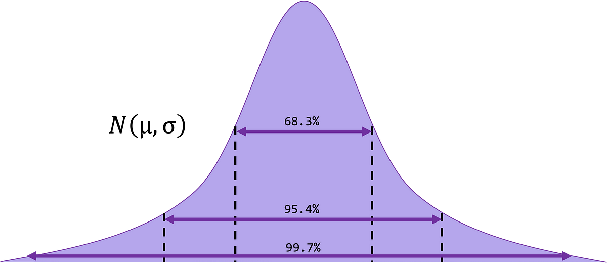
The conventional distribution (Gaussian) is a steady, symmetric, bell-shaped distribution of a variable, denoted by N(μ,σ).
The mathematical equation to characterize it’s denoted by:

and represents the likelihood density perform or p.d.f. (for brief). Imply is denoted by μ and commonplace deviation by σ.
Properties:
- Bell-shaped with the 2 tails persevering with indefinitely in each instructions
- Symmetric about heart — imply, median, and mode
- Complete space below the distribution curve is the same as 1
- Space below the curve represents likelihood

Instance. Final 12 months excessive faculties in Chicago had, 3264 feminine twelfth grade college students enrolled. The imply top of those college students was 64.4 inches and that the usual deviation was 2.4 inches. Right here the variable is top and the inhabitants consists of 3264 feminine college students attending twelfth grade. The conventional curve with the identical imply and commonplace deviation: μ = 64.4 and σ = 2.4.

Thus we are able to approximate the share of scholars between 67 anf 68 inches tall by the world below the curve between 67 and 68, the world is 0.0735 and proven on the graph as occuring between 67 and 68 inches tall.
Though we lined this in a earlier bootcamp, spaced repetition is one of the best ways to make sure recall and retention! So right here we’ve the empirical rule plotted for graphical emphasis.

- Roughly 68.3% of the information values will fall inside 1 commonplace deviation of the imply, x±1s for samples and with endpoints μ±3σ for populations
- Roughly 95.4% of the information values will fall inside 2 commonplace deviations of the imply, x±2s for samples and with endpoints μ±2σ for populations
- Roughly 99.7% of the information values will fall inside 3 commonplace deviations of the imply, x±1s for samples and with endpoints μ±3σ for populations
Totally different regular distributions have completely different means and commonplace deviations. A commonplace regular distribution is a traditional distribution with a imply of 0 and a regular deviation of 1. The notation of the p.d.f. for the usual regular distribution is:

We will see, trying on the equation above, it’s the simplification of that supplied by the p.d.f. of the conventional distribution (above). Standardization is the method by which we convert these distributions into the usual regular distribution (0,1) for comparability. We will convert the values of any usually distributed variable utilizing the equation under, which is named the z-score.


Evaluate this with the beforehand outlined p.d.f. for the conventional curve above.

Space Underneath the Customary Regular Distribution
After changing your regular distribution into a regular regular distribution, search for z-scores within the Customary Regular Distribution desk (z-table) to find out the world below the curve. We use this desk to search out the world below the curve (highlighted within the determine under) that lies (a) to the left of a specified z-score b) to the fitting of a specified z-score, and c) between two specified z-scores.

Examples.

a) Discover the world to the left of z=2.06. P(Z < 2.06) = 98.03%
b) Discover the world to the fitting of z = -1.19. P(Z>-1.19) = 88.3%
c) Discover the world between z = 1.68 and z = -1.37.
P(-1.37 < Z < 1.68) = P(Z<1.68) — P(Z < -1.37)
= 0.9535–0.0853
= 0.8682 = 86.82%
Do not forget that a t-table defaults to the LEFT….

Instance. Through the 2008 baseball season, Mark recorded his distances (in meter) for every house run and located they’re usually distributed with a imply of 100 and a regular deviation of 16. Decide the likelihood of his subsequent house run falling between 115 and 140 meters.
P(115<X<140)=? the place X = distances for every house run.
Sketch the conventional curve: X ~ N(100,16), with μ = 100 and σ = 16.
Compute the z-scores:
z1 = (115–100)/16 = 0.94
z2 = (110–100)/16 = 2.50
P(z1 < Z < z2) = ? The place Z~ N(0,1).

The world below the usual regular curve that lies between 0.94 and a pair of.50 is identical as the world space between 115 and 140 below the conventional curve with imply 100 and commonplace deviation 16, i.e. P(115<X<140) = P(0.94<Z<2.50) = P(Z<2.50) — P(Z<0.94).
The world to the left of 0.94 is 0.8264, and the world to the left of two.50 is 0.9938. the required space, is subsequently 0.9938–0.8264 = 0.1674. The possibility that Mark’s subsequent house run falls between 115 and 140 meters is 0.1674 = 16.74%.
Instance. What if you got an space below the usual regular distribution curve and requested to search out the z-score?

Assemble a traditional likelihood plot, given a dataset:

Regular likelihood plot is the plot of noticed knowledge versus regular scores. Whether it is linear, the variable is generally distributed, and if it isn’t linear, the variable shouldn’t be usually distributed. Plotting the information above, we get the plot:

Regular Q-Q Plot
A Q-Q plot (quantile-quantile plot) is a likelihood plot, which is a graphical methodology for evaluating two likelihood distributions by plotting their quantiles towards one another.
If the information are really sampled from a Gaussian distribution, the Q-Q plot shall be linear:

Code to generate the plot above:
import numpy as np
import statsmodels.api as statmod
import matplotlib.pyplot as plt#create dataset with 100 values that observe a traditional distribution
knowledge = np.random.regular(0,1,100)#create Q-Q plot with 45-degree line added to plot
fig = statmod.qqplot(knowledge, line='45')
plt.present()
The pattern means from completely different samples characterize a random variable and observe a distribution. x

A sampling distribution of pattern means is a distribution utilizing the means computed from all doable random samples of a selected measurement taken from a inhabitants. If the samples are randomly chosen with alternative, the pattern means, for probably the most half, shall be considerably completely different from the inhabitants imply μ. These variations are attributable to sampling error. Sampling error is the distinction between the pattern measure and the corresponding inhabitants measure, because of the truth that the pattern shouldn’t be an ideal illustration of the inhabitants.
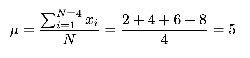
Instance. Suppose a professor gave an 8 level quiz to a small class of 4 college students. The outcomes of the quiz have been 2, 4, 6, and eight. For the sake of debate, assume that the 4 college students represent the inhabitants.
The imply of the inhabitants is:
The usual deviation of the inhabitants is:

Now, if all pattern sizes of two are taken with alternative and the imply of every pattern is discovered, the distribution is:

The imply of the pattern means is:

The usual deviation of the pattern means is:

Properties of Pattern Means
- The imply of the pattern means would be the identical because the inhabitants imply.

2. The usual deviation of the pattern means shall be smaller than the usual deviation of the inhabitants, and it is going to be equal to the inhabitants deviation divided by the sq. root of the pattern measurement. Because of this there’s much less sampling error, and is related to a bigger pattern measurement.

**The usual deviation of the pattern means is named the commonplace error of the imply**
The bigger the pattern measurement:
- the nearer the pattern imply mux approximates the inhabitants imply mu.
- the much less sampling error
- the smaller the usual deviation of the pattern means across the inhabitants imply

Distribution of pattern means for a lot of samples

- Conclusion: there shall be 95.4% of pattern implies that fall inside 2σ_xbar of every aspect of μ_xbar or μ.
- In different phrases: if we’ve 100 samples, there shall be round 95 samples means falling inside 2σ_xbar of every aspect of μ.
Confidence Interval
If we repeat the above experiment a number of occasions and every time we assemble intervals of size 2 commonplace errors to every aspect of the extimates of Xbar, then we may be assured (assume empirical rule) that 95.4% of those intervals will cowl the inhabitants parameter, μ.
If we repeat the experiment a number of occasions and assemble a number of confidence intervals, then 95.4% of those intervals embrace the inhabitants parameter, μ.
The central restrict theorem states that because the pattern measurement n will increase with out restrict, the form of the distribution of the pattern means taken with alternative from a inhabitants with imply, μ and a regular deviation σ, will strategy a traditional distribution. This distribution could have a imply μ and a regular deviation μ/sqrt(n).
Why is the central restrict theorem (CLT) so vital?
If the pattern measurement is sufficiently massive, the CLT can be utilized to reply questions on pattern means, no matter what the distribution of the inhabitants is.
That’s:

and changing to a z-score:

- When the variable from the inhabitants is generally distributed, the distribution of the pattern means shall be usually distributed, for any pattern measurement, n.
- When the variable from the inhabitants shouldn’t be usually distributed, the rule of the thumb is: a pattern measurement of 30 or extra is required to make use of a traditional distribution to approximate the pattern imply distribution. The bigger the pattern measurement, the higher the approximation shall be. That’s, want n ≥ 30 for CLT to kick in.
Abstract of z-score formulation
The primary is used to achieve details about a person knowledge level when the variable is generally distributed:

Note: This primary equation for z DEFAULTS TO THE LEFT!
The second is used once we need to acquire info when making use of the central restrict theorem a couple of pattern imply when the variable is generally distributed OR when the pattern measurement ≥ 30:

Instance. The typical variety of kilos of meat that an individual consumes per 12 months is 218.4 kilos. Assume that the usual deviation is 25 kilos and the distribution is roughly regular.
a) Discover the likelihood that an individual chosen at random consumes lower than 224 kilos per 12 months.
b) If a pattern of 40 people is chosen, discover the likelihood that the imply of the pattern shall be lower than 224 kilos per 12 months.
Resolution:
a) The query asks about a person individual.

b)The query considerations the imply of the pattern with a measurement 40.

The big distinction between these two chances is because of the truth that the distribution of pattern means is way much less variable than the distribution of particular person knowledge values. (Observe: A person individual is the equal of claiming n=1).
Recall that the binomial distribution is set by n (the variety of trials) and p (the likelihood of success). When p is roughly 0.5, and as n will increase, the form of the binomial distribution turns into much like that of a traditional distribution.
When p is near 0 or and n is comparatively small, a traditional approximation is inaccurate. As a rule of thumb, statisticians usually agree {that a} regular approximation needs to be used solely when n*p and n*q are each larger than or equal to five, i.e. np≥5 and nq≥5.

import math
import matplotlib.pyplot as pyplotdef binomial(x, n, p):
return math.comb(n, x) * (p ** x) * ((1 - p) ** (n - x))n = 50
p = 0.5
binomial_list = []
keys = []for x in vary(50):
binomial_list.append(binomial(x, n, p))for y in vary(50):
keys.append(y)pyplot.bar(x=keys, top=binomial_list)
pyplot.present()
A correction for continuity is a correction employed when a steady distribution is used to approximate a discrete distribution.

For all circumstances, μ=n*p, σ=sqrt(n*p*q), n*p≥5, n*q≥5
Step-wise Course of for the Regular Approximation to the Binomial Distribution
- Examine to see whether or not the conventional approximation can be utilized
- Discover the imply μ, and commonplace deviation σ
- Write the issue utilizing likelihood notation, e.g. P(X=x)
- Rewrite the issue leveraging the continuity correction issue and present the corresponding AUC of the conventional distribution
- Calculate corresponding z values
- Resolve!
Instance. {A magazine} reported that 6% of Individuals take a look at their telephone whereas driving. If 300 drivers are chosen at random, discover the precise likelihood that 25 of them take a look at their telephone whereas driving. Then use the conventional approximation to search out the approximate likelihood.
p=0.06, q=0.94, n=300, X=25
The actual likelihood utilizing the binomial approximation:

Regular approximation strategy:
- Examine to see whether or not a traditional approximation can be utilized. n*p=300*0.06 = 18, n*q = 300*0.94 = 282
Since n*p ≥ 5, and n*q ≥ 5, the conventional distribution can be utilized - Discover the imply and commonplace deviation

3. Write the issue in likelihood notation P(X=25).
4. Rewrite the issue by utilizing the continuity correction issue.
P(25–0.5 < X < 25 + 0.5) = P(24.5 < X < 25.5)
5. Discover the corresponding z values:

6. Resolve:

The likelihood that 25 folks learn the newspaper whereas driving is 2.27%.
On this bootcamp, we’ve continued within the vein of likelihood concept now together with work to introduce Bayes theorem and the way we are able to derive it utilizing our beforehand realized guidelines of likelihood (multiplication concept). You will have additionally realized how to consider likelihood distributions — Poisson, Bernoulli, Multinomial and Hypergeometric. Look out for the following installment of this sequence, the place we are going to proceed to construct our data of stats!!
Earlier boot camps within the sequence:
#1 Laying the Foundations
#2 Middle, Variation and Place
#3 Likelihood… Likelihood
#4 Bayes, Fish, Goats and Automobiles
All pictures except in any other case acknowledged are created by the creator.
