Including up SHAP values of categorical options which were remodeled with one-hot encodings
Categorical options have to be remodeled earlier than they can be utilized in a mannequin. One-hot encoding is a standard manner to do that: We find yourself with a binary variable for every class. That is superb till it involves understanding the mannequin utilizing SHAP. Each binary variable can have its personal SHAP worth. This makes it obscure the general contribution of the unique categorical function.
A easy method is so as to add the SHAP values for every of the binary variables collectively. This may be interpreted because the SHAP worth for the unique categorical function. We are going to stroll you thru the Python code for doing this. We are going to see that we’re ready to make use of the SHAP aggregation plots. Nonetheless, these are restricted in relation to understanding the character of relationships of the explicit options. So, to finish we present you the way boxplots can be utilized to visualise the SHAP values.
In case you are unfamiliar with SHAP or the python package deal, I recommend studying the article under. We go in depth on interpret SHAP values. We additionally discover a few of the aggregations used on this article.
To show the issue with categorical options, we might be utilizing the mushroom classification dataset. You’ll be able to see a snapshot of this dataset in Determine 1. The goal variable is the mushroom’s class. That’s if the mushroom is toxic (p) or edible (e). You’ll find this dataset in UCI’s MLR.

For mannequin options, we now have 22 categorical options. For every function, the classes are represented by a letter. For instance odor has 9 distinctive categories- almond (a), anise (l), creosote (c), fishy (y), foul (f), musty (m), none (n), pungent (p), spicy (s). That is what the mushroom smells like.
We’ll stroll you thru the code used to analyse this dataset and you will discover the total script on GitHub. To begin, we might be utilizing the Python packages under. Now we have some widespread packages for dealing with and visualising knowledge (traces 2–4). We use the OneHotEncoder for reworking the explicit options (line 6). We use xgboost for modelling (line 8). Lastly, we use shap to know how our mannequin works (line 10).
We import our dataset (line 2). We’d like a numerical goal variable so we remodel it by setting toxic = 1 and edible = 0 (line 6). We additionally get the explicit options (line 7). We don’t use the X_cat dataset for modelling however it’s going to come in useful in a while.
To make use of the explicit function we additionally want to remodel them. We begin by becoming an encoder (traces 2–3). We then use this to remodel our categorical options (line 6). For every categorical function, there might be a binary function for every of its classes. We create function names for every of the binary options (traces 9 to 10). Lastly, we put these collectively to create our function matrix (line 12).
In the long run, we now have 117 options. You’ll be able to see a snapshot of the function matrix in Determine 2. For instance, you may see that cap-shape has now been remodeled into 6 binary variables. The letters on the finish of the function names come from the unique function’s classes.

We prepare a mannequin utilizing this function matrix (traces 2–5). We’re utilizing an XGBClassifier. The XGBoost mannequin consists of 10 timber and every tree has a most depth of two. This mannequin has an accuracy of 97.7% on the coaching set.
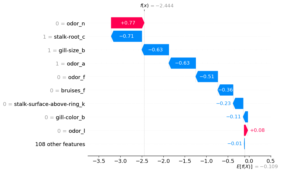
At this level, we need to perceive how the mannequin is making these predictions. We begin by calculating the SHAP values (traces 2–3). We then visualise the SHAP values of the primary prediction utilizing a waterfall plot (line 6). You’ll be able to see this plot in Determine 3.
You’ll be able to see that every binary function has its personal SHAP worth. Take odor for instance. It seems 4 instances within the waterfall plot. The truth that odor_n = 0 will increase the likelihood that the mushroom is toxic. On the identical time, odor_a = 1, odor_f = 0 and odor_I = 0 all lower the likelihood. It’s not clear what the general contribution of the mushroom’s odor is. Within the subsequent part, we are going to see that it does turn out to be clear once we add all the person contributions collectively.
Let’s begin by exploring the shap_values object. We print the item within the code under. You’ll be able to see within the output under that’s made of three parts. Now we have the SHAP values (values) for every of the predictions. knowledge provides the values for the binary options. Every prediction will even have the identical base worth (base_values). That is the common predicted log odds.
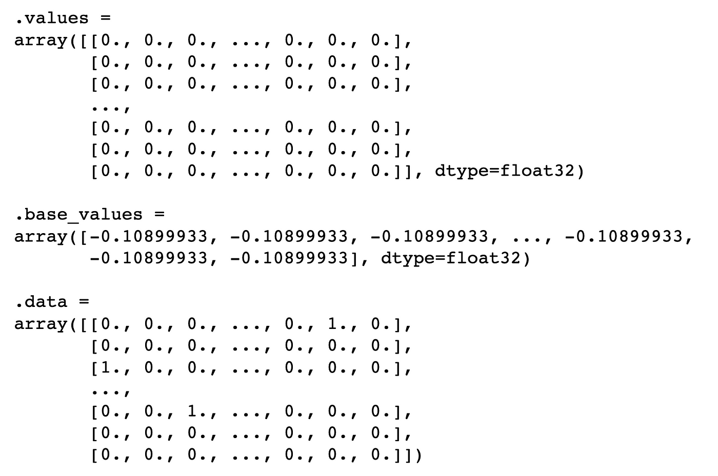
We will take a better have a look at the SHAP values for the primary prediction by printing them under. There are 117 values. One for every binary variable. The SHAP values are in the identical order because the X function matrix. Keep in mind, the primary categorical function, cap-shape, had 6 classes. This implies the primary 6 SHAP values correspond to the binary options from this function. The subsequent 4 correspond to the cap-surface options and so forth.

We need to add the SHAP values for every categorical function collectively. To do that we begin by creating the n_categories array. This comprises the variety of distinctive classes for every categorical variable. The primary quantity within the array might be 6 for cap-shape then 4 for cap-surface and so forth…
We use n_categories to separate the SHAP worth arrays (line 5). We find yourself with an inventory of sublists. We then sum the values inside every of those sublists (line 8). By doing this we go from 117 SHAP values to 22 SHAP values. We do that for each remark within the shap_values object (line 2). For every iteration, we add the summed shap values to the new_shap_values array (line 10).
Now, all we have to do is exchange the unique SHAP values with the brand new values (line 2). We additionally exchange the binary function knowledge with the class letters from the unique categorical options (traces 5–6). Lastly, we exchange the binary function names with the unique function names (line 9). It is very important cross these new values as arrays and lists respectfully. These are the info sorts utilized by the shap_values object.
The up to date shap_values object can be utilized similar to the unique object. Within the code under we plot the waterfall for the primary remark. You’ll discover this code is strictly the identical as earlier than.
You’ll be able to see the output in Determine 4. We now have 22 SHAP values. You may also see the function values on the left have been changed with the class labels. We mentioned the odor function earlier than. Now you can clearly see the general contribution of this function. It has decreased the log odds by 0.29.
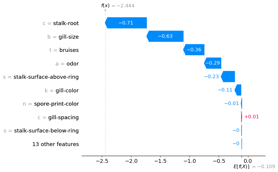
Within the above plot, we now have odor = a. This tells us the mushroom had an “almond” scent. We should always keep away from decoding the plot as “the almond scent has decreased the log odds”. Now we have summed a number of SHAP values collectively. Therefore, we must always interpret it as “the almond scent and lack of different scents has decreased the log odds”. For instance, trying on the first waterfall plot the dearth of a “foul” odor (odor_f = 0) has additionally decreased the log odds.
Earlier than we transfer on to aggregations of those new SHAP values, it’s price discussing some principle. The explanation we’re ready to do that with SHAP values is due to their additive property. That’s the common prediction (E[f(x)]) plus the entire SHAP values equal the precise prediction (f(x)). By including some SHAP values collectively we don’t intervene with this property. This is the reason f(x) = -2.444 is similar in each Determine 3 and Determine 4.
Imply SHAP
Like with the waterfall plot, we will use the SHAP aggregations similar to with the unique SHAP values. For instance, we use the imply SHAP plot within the code under. Determine 5, we will use this plot to spotlight necessary categorical options. For instance, we will see that odor tends to have giant constructive/ unfavourable SHAP values.

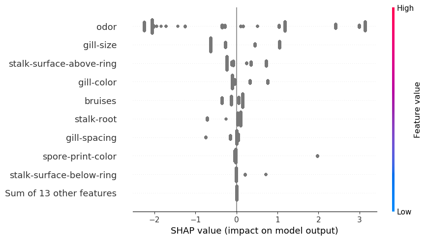
Beeswarm
One other widespread aggregation is the beeswarm plot. For steady variables, this plot is helpful as it might assist clarify the character of the relationships. We will see how SHAP values are related to the function values. Nonetheless, for the explicit options, we now have changed the function values with labels. In consequence, in Determine 6, you may see the SHAP values are all given the identical color. We have to create our personal plots to know the character of those relationships.
SHAP Boxplot
A method we will do that is by utilizing boxplots of the SHAP values. In Determine 7, you may see one for the odor function. Right here we now have grouped the SHAP values for the odor function base on the odor class. You’ll be able to see {that a} foul scent results in larger SHAP values. These mushrooms usually tend to be toxic. Please don’t eat any bad-smelling mushrooms! Equally, mushrooms with no scent usually tend to be edible. A single orange line means all of the SHAP values for these mushrooms have been the identical.

We create this boxplot utilizing the code under. We begin by getting the odor SHAP values (line 2). Keep in mind these are the replace values. For every prediction, there might be just one SHAP worth for the odor function. We additionally get the odor class labels (line 3). We cut up the SHAP values primarily based on these labels (traces 6-11). Recently, we use these values to plot a boxplot for every of the odor classes (traces 27–32). To make the chart simpler to interpret, we now have additionally changed the letter with the total class names (traces 14–24).
In follow, it’s doubtless that solely a handful of your options might be categorical. You will have to replace the above course of to solely sum the explicit ones. You could possibly additionally provide you with your individual manner of visualising the relationships of those options. In case you provide you with one other manner I’d love to listen to about it within the feedback.
I’d additionally have an interest to know how function dependencies will have an effect on this evaluation. By definition, the remodeled binary options might be correlated. This could impression the SHAP worth calculation. We’re utilizing TreeSHAP to estimate the SHAP values. My understanding is that these aren’t impacted by dependencies as a lot as KernelSHAP. I’m to listen to your ideas within the feedback.
