
A brief information on utilizing Seaborn’s Pairplot in Python

The Seaborn Pairplot permits us to plot pairwise relationships between variables inside a dataset. This creates a pleasant visualisation and helps us perceive the information by summarising a considerable amount of information in a single determine. That is important after we are exploring our dataset and making an attempt to change into acquainted with it.

Because the saying goes, an image paints a thousand phrases.
On this brief information we shall be masking methods to create a fundamental pairplot with Seaborn, and management the aesthetics of it together with the determine measurement and styling.
The dataset we’re utilizing for this tutorial is a subset of a coaching dataset used as a part of a Machine Studying competitors run by Xeek and FORCE 2020 (Bormann et al., 2020). It’s launched below a NOLD 2.0 licence from the Norwegian Authorities, particulars of which could be discovered right here: Norwegian Licence for Open Authorities Information (NLOD) 2.0.
The complete dataset could be accessed on the following hyperlink: https://doi.org/10.5281/zenodo.4351155.
The target of the competitors was to foretell lithology from current labelled information utilizing nicely log measurements. The complete dataset consists of 118 wells from the Norwegian Sea.
Moreover, you’ll be able to obtain the subset of the information used on this tutorial together with the pocket book from the GitHub Repository:
I’ve additionally launched the next video which can be of curiosity to you.
Step one is to import the libraries that we’ll be working with. On this case we’re going to be utilizing Seaborn which is our information visualisation library and pandas, which shall be used to load in our information and retailer it.
import seaborn as sns
import pandas as pd
To model the Seaborn plots, I’ve set the model to darkgrid
# Setting the stying of the Seaborn determine
sns.set_style('darkgrid')
Subsequent I’ve loaded in some nicely log information from the Drive 2020 Machine Studying competitors that targeted on predicting lithology from nicely log measurements. Don’t fear if you’re not acquainted with this dataset as what I’m going to indicate you could be utilized to virtually every other dataset.
df = pd.read_csv('Information/Xeek_Well_15-9-15.csv')# Take away excessive GR values to help visualisation
df = df[df['GR']<= 200]
Along with loading information, I’ve eliminated Gamma Ray (GR) values above 200 API to help within the visualisation of this information. Ideally, it is best to examine why these factors are studying excessive earlier than eradicating them.
Now that the information has been loaded, we are able to transfer onto creating our first pairplot. To get a pairplot for all the numeric variables inside our dataset we merely name upon sns.pairplot and go in our dataframe — df.
sns.pairplot(df)
As soon as this runs, we get again a big determine containing many subplots.

If we take a more in-depth take a look at the produced determine, we are able to see that we’ve got all of our variables proven alongside the y and x axis. Alongside the diagonal we’ve got a histogram displaying the distribution of every of the variables.
Immediately we’ve got a single determine that can be utilized to offer a pleasant condensed abstract of our dataset.
If we solely need to present a handful of variables from our dataframe, we first must create an inventory of the variables we need to examine:
cols_to_plot = ['RHOB', 'GR', 'NPHI', 'DTC', 'LITH']
Within the instance above I created a brand new variable cols_to_plot and assigned it to an inventory containing RHOB, GR, NPHI, DTC and LITH. The primary 4 of those are numeric, and the final is categorical, which can use later.
We will then name upon our pairplot and go the dataframe with this checklist like so:
sns.pairplot(df[cols_to_plot])
Once we run this, we get again a a lot smaller determine with solely the variables we’re eager about.

As a substitute of getting a histogram alongside the diagonal, we are able to swap it out for a kernel density estimate (KDE), which offers us with one other strategy to view the distribution of the information.
To do that we merely add within the key phrase argument: diag_kind is the same as kde like so:
sns.pairplot(df[cols_to_plot], diag_kind='kde')
Which returns the next determine:

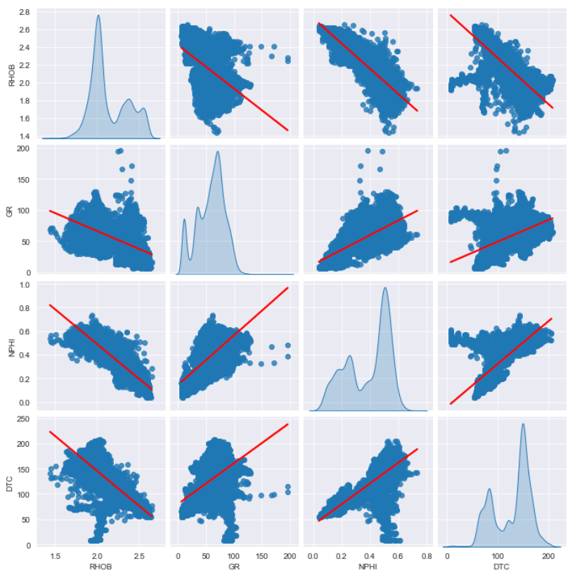
If we need to establish relationships throughout the scatter plots, we are able to apply a linear regression line, which is just achieved by including the key phrase: variety and assigning it to 'reg' .
sns.pairplot(df[cols_to_plot], variety='reg', diag_kind='kde')
Once we run this we’ll now see we’ve got a partial line showing on every of the scatter plots

Nevertheless, as the road color is identical as the purpose color we have to change this to make it extra seen.
We will do that by including the plot_kws key phrase, after which we have to go in a dictionary, which can then include line_kws, which then will get handed one more dictionary object for our colour which we’ll set to pink.
# Use plot_kws to vary regression line color
sns.pairplot(df[cols_to_plot], variety='reg', diag_kind='kde',
plot_kws={'line_kws':{'colour':'pink'}})
Once we run the code, we get again a pairplot with a pink line, which makes it a lot simpler to see.
If we’ve got a categorical variable inside our dataframe, we are able to use that to visually improve the plots and see tendencies and distributions for every class.
Inside this dataset we’ve got a variable known as LITH, which represents completely different lithologies which have been recognized from the nicely log measurements.
If we’re utilizing a subset of our dataframe, we have to make sure that the cols_to_plot line accommodates the variable we need to color the information with.
To make use of that variable, all we do is add a hue argument, and go within the 'LITH' column from our checklist and run the code.
sns.pairplot(df[cols_to_plot], hue='LITH')
What we get again is a pairplot colored by every of the classes inside that variable.
If we’ve got a more in-depth take a look at the information, we’ve got Shales in blue, sandstone in inexperienced and limestone in pink, and from these we are able to achieve some insights into our information. For example, we we take a look at shale, we are able to see we’ve got a big peak within the GR variable at round 100 API, and a smaller pink peak for Chalk round 25 API. So immediately we are able to get an thought of the vary for every of the lithologies.
Now that we’ve got lined the fundamentals of the pairplot, we are able to now take issues to the following degree and begin styling our plot.
First up we’ll begin by altering the properties of the diagonal histogram. We will change the diagonal styling through the use of the diag_kws key phrase and passing in a dictionary of what we need to change.
On this instance, we’ll change the color by passing in a colour key phrase and setting it to pink.
sns.pairplot(df[cols_to_plot], diag_kws={'colour':'pink'})
Once we run this, we get again the next plot:

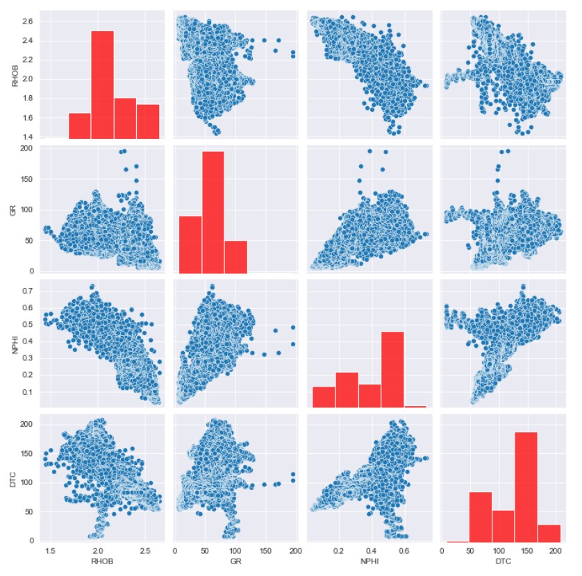
As this can be a histogram, we are able to additionally change the variety of bins being displayed. Once more, that is achieved by passing in a dictionary containing the property we need to change, which on this case is bins.
We’ll set this to five and run the code.
sns.pairplot(df[cols_to_plot], diag_kws={'colour':'pink', 'bins':5})
Which returns this determine with 5 bins and the information colored in pink.
If we need to model the factors, we are able to achieve this utilizing the plot_kws key phrase, and passing in our dictionary containing colour , which we’ll set to inexperienced.
sns.pairplot(df[cols_to_plot], diag_kws={'colour':'pink'},
plot_kws={'colour':'inexperienced'})

And if we need to change the purpose measurement, we merely add the s key phrase argument into the dictionary. This can scale back the dimensions of the factors.

Lastly, we are able to management the dimensions of our determine in a quite simple method by including within the key phrase argument peak which on this instance we’ll set to 2. Once we run this code, we’ll see we now have a a lot smaller plot.
sns.pairplot(df[cols_to_plot], peak=2)
We will additionally use the side key phrase argument to regulate the width. By default that is set to 1, but when we set it to 2, it means we’re setting the width to twice the dimensions of the peak.
sns.pairplot(df[cols_to_plot], peak=2, side=2)

The Seaborn Pairplot is a good information visualisation device that helps us change into acquainted with our information. We will plot a considerable amount of information on a single determine and achieve an understanding of it in addition to develop new insights. Positively a plot to maintain in your information science toolbox.
