Commonplace plots for binary classifications at the moment are obtainable within the binclass-tools bundle

I lately introduced the discharge of a Python bundle helpful for the evaluation of binary classifications. Particularly, the necessity to develop this bundle arose from the problem of analyzing imbalanced binary classifications. Utilizing interactive plots for confusion matrix and value evaluation proved to be important for finding out mannequin efficiency, so the Python binclass-tools bundle was created, as I highlighted in my following article:
For the reason that purpose of this Python bundle is to supply the top consumer with a set of helpful instruments for binary classification fashions, fundamental plots have been added, together with the confusion matrix and value plots, that are used to measure mannequin efficiency.
Usually, to grasp how a binary classification mannequin performs, along with analyzing its confusion matrix, the analyst plots the well-known Receiver Working Traits (ROC) and the Precision-Recall (PR) curves. This text is past the scope of explaining how the above curves are constructed. Extra particulars on how to do that could be discovered within the references. What’s fascinating to level out is that as of at this time it’s also doable to plot the above two curves very simply due to the binclass-tools bundle.
As soon as the classifier is educated, one can simply compute the vector containing the prediction rating obtained by passing the take a look at dataset to the predict_proba of the classifier (outcome within the variable test_predicted_proba ). Then, one can use the curve_ROC_plot perform of the bundle to get the ROC curve, passing the anticipated scores and the corresponding true labels:
area_under_ROC = bc.curve_ROC_plot(
true_y = y_test,
predicted_proba = test_predicted_proba)
The perform, along with the plot, additionally returns the worth of the realm beneath the ROC curve. The ensuing plot is as follows:

Because of the interactivity of the plot, you’ll be able to view the values of the brink, False Optimistic Charge (FPR) and True Optimistic Charge (TPR) for every level on the curve within the tooltip.
Equally, it’s doable to plot the Precision-Recall curve with the next easy code:
area_under_PR = bc.curve_PR_plot(
true_y= y_test,
predicted_proba = test_predicted_proba,
beta = 1)
Along with returning the realm beneath the PR curve, the perform additionally returns the next plot:

Once more, the interactivity of the plot lets you discover the precision and recall values for every threshold. The tooltip additionally exhibits the fᵦ-score worth (with the β worth handed as a parameter to the perform), a metric outlined via precision and recall and infrequently used to judge mannequin efficiency. Furthermore, the plot accommodates iso-fᵦ curves, which establish for comfort the factors at which fᵦ values are fixed.
In each the ROC and PR curves the baseline (dummy curve of a naïve mannequin that guesses the goal class randomly) is plotted.
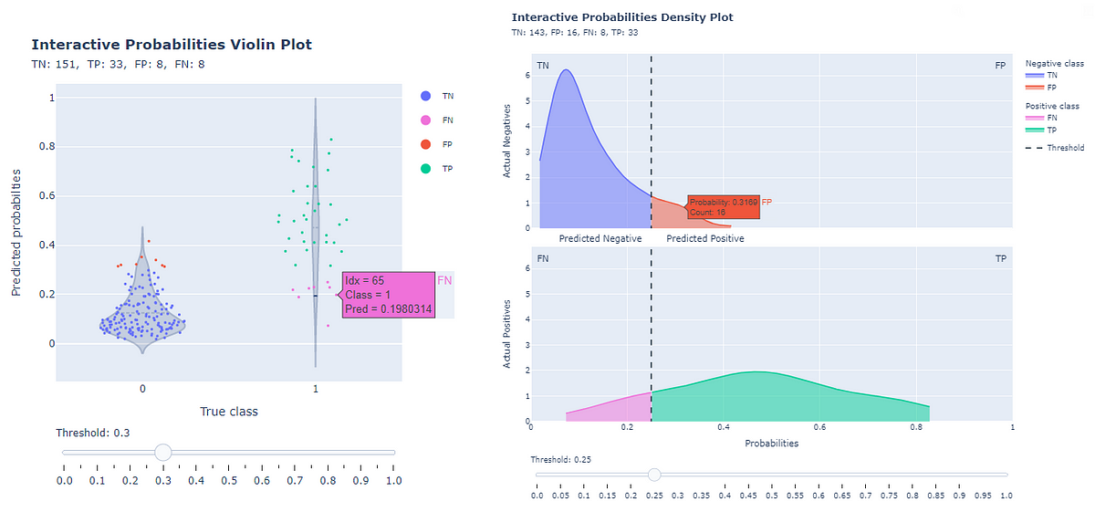
Distributions of predict_proba scores for every of the 2 goal lessons could be studied utilizing the Interactive Chances Distribution Plot, which makes use of violin plots to finest signify them. The plot in query is used to reply the query, “How are the chance rating values distributed for every of the anticipated goal lessons?”.
A really handy function of this interactive plot is the slider that enables the brink of the classifier to be modified. This enables the subsets of predictions related to the confusion matrix classifications (TP, TN, FP, FN) to be displayed as factors above the distribution plots of the scores for every goal class:

Hovering over the factors produces a tooltip that accommodates the road quantity indicator of the statement related to the purpose (idx), the true class of the statement (class), and the worth of the predict_proba rating related to the statement (pred). By hovering the mouse over the facet edges of the plot, we as a substitute get the quartiles data for every of the 2 violin plots. Completely different colours distinguish the totally different classes of the confusion matrix.
Violin plots help you get a “top-down” view of the distributions of predictions damaged down by goal lessons. If, alternatively, you need to view the identical distributions as “profile photographs” (as they’re often displayed), you’ll be able to generate the Interactive Chances Density Plot due to the brand new predicted_proba_density_curve_plot perform, smoothing the histogram bins utilizing Gaussian or KDE strategies, utilizing this code:
threshold_step = 0.05
curve_type = 'kde' #'kde' is the default worth, 'regular' in any other casebc.predicted_proba_density_curve_plot(
true_y = y_test,
predicted_proba = test_predicted_proba,
threshold_step = threshold_step,
curve_type = curve_type)
The output you get is an interactive plot that additionally has the slider for the brink, the step of which is outlined within the name to the earlier perform:

Every of the 2 sub-graphs on this plot is split into two zones by the vertical dashed line figuring out the brink. Every of the 2 sub-graphs on this plot is split into two zones by the vertical dashed line figuring out the brink. 4 zones are thus fashioned, every related to a confusion matrix classification (TN, FP, FN, TP). Subsequently, the tooltip highlights the main points of every particular person zone, displaying each the predict_proba rating and the variety of predictions that fall into that particular classification for that particular threshold.
Beginning with launch 0.3.0, the Python binclass-tools bundle introduces 4 new interactive plots:
- Interactive Receiver Working Traits (ROC) curve
- Interactive Precision-Recall (PR) curve
- Interactive Chances Distribution Plot
- Interactive Chances Density Plot
With the brand new model, the binclass-tools bundle could be thought of fairly full for finding out the efficiency of a binary classifier.
Among the particulars you will discover within the Precision-Recall curve and Chances Distribution Plot have been impressed by the plot-metric bundle by Yohann Lereclus and Pi Esposito:
- Understanding AUC — ROC Curve | by Sarang Narkhede | In the direction of Information Science
- Precision-Recall Curves. Typically a curve is value a thousand… | by Doug Steen | Medium
- Violin Plots 101: Visualizing Distribution and Chance Density | Mode
- In-Depth: Kernel Density Estimation | Python Information Science Handbook (jakevdp.github.io)
