
How laborious can it’s to show a machine to generate a single level

This text describes the creation of a Generator — Discriminator pair, that will be constant and sturdy (kind of). What’s extra, I aimed to get a particular Discriminator operate, which might make sure the Generator’s constant studying (see plot under).
The duty for the only GAN could be to generate some extent. A single quantity, say “1.” The Generator could be a single neuron with one weight and one bias worth. Thus, the Discriminator thus must be bell-shaped, like this:

The worth “1” is taken into account actual, the values near “1” are considerably more likely to be actual; the values additional away — in all probability faux.
I ought to begin this part by describing what Generator and Discriminator ought to be like and why they need to be like this.
First, let’s assume once more about what a Generator is. It’s a operate that transforms a random enter right into a real-looking sign. As described within the introduction, the real looking sign might be a single worth “1.” For the enter, I’ll take a random worth between -1 and +1.
The operate itself might be linear, since this instance goals to be easy:
y = w * x + b
The place y is the output, x is the enter; w is neural community weight, and b — is its bias. The answer to the issue could be:
w = 0
b = 1
On this case, it doesn’t matter what “x” is, “y” is at all times “1.” Graphically it’s represented by a vertical line, as proven within the plot under.
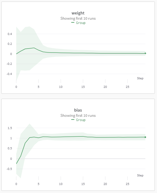
There are quite a lot of plots on this article that present coaching processes titled as “weight” and “bias.” These values signify the “w” and “b” I’ve simply described. So when wanting on the plots, we should always really feel joyful when the “weight” converges to 0 and the “bias” — to 1.
Second, the Discriminator. That is one other operate, which outputs a likelihood of its enter being genuine. In our instance, it ought to output a worth near “1” given the enter “1,” and in any other case ought to output “0.” For the GAN community, it additionally acts as a loss operate for the Generator, so it ought to be easy. Here’s a plot of each Generator and Discriminator I count on to get:

By way of formulation, the Discriminator could be so simple as potential. But it could possibly’t be linear, since we intention to get a bell form. So the only potential answer could be a multilayer perceptron with two hidden nodes:
By the best way, if I need to see what my Generator and Discriminator features seem like, I’d merely move a spread of numbers by means of them:
That is the truth is how I obtained the plots above.
Earlier than we get to the primary coaching, I’d like to debate how the mannequin might be educated and the way I’m going to visualise it. Check out the next picture:

This picture reveals the Generator and Discriminator on the very starting of the coaching, so their parameters are random.
The operate represented by the blue line is supposed to rework a random enter into a sensible worth (now it outputs random values as properly, because it’s untrained). So for instance, if we generated random values [-2.05, 0.1, 2.5] this operate would remodel them into (roughly) [-0.2, 0.3, 0.49]:

These values are then handed to the Discriminator (word the size distinction, 2 squares per worth on the vertical axis vs 1 sq. per worth on the horizontal):

The scores outputted by the Discriminator are then collected. The process is repeated with the actual worth:

The typical output could be 0.48 for the faux values and 0.56 for the actual ones. After that, each Generator and Discriminator will take totally different actions to be able to prepare.
Discriminator’s standpoint.
The Discriminator tries to make the actual and pretend values extra distinguishable by their scores. On this case, it may be achieved by making the operate steeper:

Chances are you’ll discover that I’m not defining what’s “higher” within the picture above. Later I’ll use binary cross-entropy for this goal, nevertheless it doesn’t calculate the common of uncooked outputs. Don’t pay a lot consideration to it now, because it’s a tough illustration of the method. Even the numbers on this complete part are made up.
Generator’s standpoint.
The Generator, in its flip, tries to replace its operate in a approach that when the generated values are handed by means of the Discriminator, their rating is greater. It may be achieved by merely producing bigger values:

Observe that for a similar enter [-2.05, 0.1, 2.5], the output is bigger: [0.2, 0.4, 0.75]. For the brand new values the Discriminator outputs in common 0.51, which is best.

Observe that the inputs within the decrease picture are shifted to the correct, in comparison with the highest picture.
Combining the coaching step for each fashions, we get the next transition:

The method is then repeated with new random values because the Generator enter. The general coaching passes the levels proven within the picture under.

Since we could have quite a lot of small steps like these, it’s handy to mix them into an animation, which might seem like the next:
I’ll use such animations so much, for demonstration functions. The code that generates will probably be described under.
We begin with the fashions’ code, since I’ve described them within the earlier part. That is basically the formulation above, remodeled in PyTorch code:
This code might be saved within the fashions.py file. So every time I import the fashions, I imply this code.
The coaching code follows subsequent, and this can be a bit difficult. We have to make two passes by means of the info: one for the Generator coaching and one for the Discriminator. I’ll do it in a easy approach. I’ll make them take turns. The Generator will wait whereas the Discriminator is coaching and vice versa:
As for the loss operate, I gained’t use the traditional GAN loss, simply to make it less complicated to grasp and to point out that it doesn’t need to be like this. Nonetheless, the thought behind the loss will stay the identical. The Generator desires the Discriminator to output 1 given its output:
By random_input I’ll take values from 0 to 1 generated the next approach:
The Discriminator collects the output from the Generator and the actual values, and tries to separate them:
The remainder of the code is a daily routine:
The code already accommodates logging, which is described under.
There’s one factor I’d like so as to add to the coaching — make it to generate animation, the one which is described in part “1.2 GAN coaching.” Apart from that it appears cool, it offers a great understanding of what’s going on inside. And what’s good about such a easy mannequin — we are able to afford this sort of visualization.
The kind of animation I might be utilizing is matplotlib’s FuncAnimation. The concept is that I create a determine and a operate that updates the determine; the library will name this operate for each body, and generate an animation:
On some methods, there is probably not current some libraries wanted for producing a video. On this case, one might try to generate GIFs as a substitute:
Other than the animation logs, I need to watch how the load and bias of the Generator change, to see if the coaching strikes in the correct course. I exploit Weights & Biases on this instance, however different selections, like MlFlow, are additionally acceptable.
The coaching code produces the next coaching course of (I various studying charges for the fashions and run the code with totally different random seeds):

Observe that the proper course of would find yourself with the load set to “0” and the bias to “1.”
The trainings had been principally profitable, a few of them depicted under:

However there are a few unhealthy examples:

By way of visible illustration, the GIFs, listed here are some examples:

Since many of the trainings reached their goal, this code could also be thought-about “working”, however one might not agree with it. Let’s see what’s flawed and the way we are able to repair it.
There are solely two issues that make me query whether or not my coaching is appropriate. First, it does fail typically, so it should be considerably unstable. Second, is the Discriminator operate. There are solely a handful of instances the place it appears the best way I used to be anticipating. Let’s look at the issues I encountered.
In some unspecified time in the future, the Generator begins to output real looking values (as a result of we prepare it to take action) and there’s no approach for the Discriminator to search out the distinction. However the community doesn’t know this, so it continues the coaching. Because the enter is already real looking, it’s invalid. And everyone knows that the networks educated on invalid information are insufficient.
Making an attempt to determine the issue, I took a Generator from one of many failed instances and plotted a number of the Discriminator parameters together with a loss worth it produce.
The Generator has already produced values near actual, one thing within the vary [-0.59, +0.62].
What I discovered was slightly shocking, as a result of a greater Discriminator operate (that I, as a human, know is best) — in actuality gave worse loss values:

This was as a result of the values which have been generated had been near actual. So the proper Discriminator would consider them roughly the identical, with solely a minor distinction. However, the inaccurate Discriminator would have barely improved its efficiency by making radical adjustments like within the plot above.
What first got here to thoughts was that this Discriminator evaluates the actual examples as actual with a 0.5 likelihood. That is one thing straightforward to repair by giving weights to the loss operate. This experiment is described within the part under, with all the opposite experiments. However lengthy story quick, it didn’t work.
Earlier than transferring on to the answer that labored, I’d prefer to share the outcomes of the experiments, primarily based on the assumptions I made above.
- Loss operate easing
The present cross-entropy loss operate desires the community output to be 0 and 1, which makes the values earlier than activation (sigmoid) very massive constructive or unfavourable values. Since our Discriminator is supposed to be versatile, massive values usually are not one thing we would like. One answer for that’s to make the targets not so excessive. I’d set them to 0.1 and 0.9 as a substitute of 0 and 1. In order that the weights usually are not compelled to be massive. Ultimately, all we want from the Discriminator are gradients.
In code, I’ll change the goal for the discriminator to this (with easing parameter being various):
Which after coaching once more, will yield these curves:

This appears extra secure, however I nonetheless don’t just like the GIFs:

2. Weighting the actual examples
In code, I’ll set much less weight to the faux examples (right here weight is a small worth):
Ran the coaching once more, obtained the next picture. In brief, didn’t work:

3. Weight decay
One of many causes the coaching might fail is that the Discriminator might go too far attempting to categorise the output from an un-trained Generator. Particularly if the Discriminator learns considerably quicker than the Generator.
So given a place to begin like this

The Discriminator will shortly study a operate like this:

Observe the sharpness of the Discriminator operate. Which means its weights are massive, and the gradients exterior the (small) curvy space are near zero; so the mannequin learns very slowly (if in any respect).
So the thought was so as to add a weight decay to stop the mannequin from reaching this state:
Which supplies the next coaching stats:

And is visualized as follows:


One might even see that this technique is succesful to enhance the coaching, however I’m nonetheless not glad with the coaching course of.
Let’s have a look once more on the scenario when the Generator outputs real looking solutions however the Discriminator nonetheless has to study one thing. One answer to this downside could be to make the Generator’s output invalid. Solely throughout the Discriminator coaching, after all. This could resemble some type of dropout. This could work, as a result of the precise dropout works, however there are too few parameters within the Generator. If we zero out certainly one of them, the output will change an excessive amount of.
The answer I’ve give you entails including Gaussian noise to the Generator’s parameters (to the load and bias). In that approach, even when the Generator is completely appropriate, it should generate barely invalid information for the Discriminator, in order that it could possibly study:
The remaining downside is that the coaching goes too noisy for the reason that gradients change quickly with every optimization step. So I made a decision to make a collection of evaluations with a unique noise, earlier than the optimization — some type of a batch contained in the batch:
This improves the coaching course of:

And on the finish generates a phenomenal Generator operate:

However nonetheless, some trainings didn’t go properly. Listed below are the coaching logs:

I’ve to say that the scenario I’ve described within the “Loss operate doesn’t work” part might also seem right here if the noise of the weights is simply too small. It simply doesn’t push the mannequin far sufficient to generate an clearly flawed instance. So I made a decision to extend the noise degree:
NOISE_SCALE = 1.5 # As a substitute of 0.5
This step improved the stats, however there have been nonetheless fails remaining:
The subsequent enchancment I utilized was the load decay, for the explanations I described above within the “Organising experiments” part beneath “3. Weight decay.” This yielded the next stats:

Which suggests no failing runs in any respect. The load decay has a facet impact that the Discriminator operate turns into smoother, so the GIFs look attractive:

For my instance, I took weight decay worth as 1e-1:
However take into account that it is dependent upon the load noise degree. If it’s small, you might have to lower the load decay. In any other case, the Discriminator will go flat.
The total up to date code would look as follows:
This code appears to be constant and sturdy, at the least for such a easy activity. Some parameters nonetheless must be tuned, like inner batch dimension or weight decay worth, however general, I’m glad with the consequence. The ultimate model of the code doesn’t require as a lot wrestle as the primary one, so I contemplate it successful.
Hope it was useful, joyful coding!
