
That is the right way to estimate the parameters of your Chirplet, utilizing Python

One of the widespread operations of Sign Processing is to remodel the sign. The explanation why we do that’s that it isn’t at all times true that the simplest technique to carry out operations in your sign is by it and analyzing it in its pure area*.
* I’ll check with the pure area as the unique area of the sign. For instance, if the sign is a time collection, the pure area is the 2D one the place the x is the time and the y is the sign worth
In my newest medium article, I defined the distinction between the Fourier Remodel and the Chirplet one.
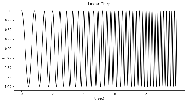
The important thing distinction between these two indicators is that the Fourier Remodel is used for indicators which have non-dependency between time and frequency (Frequency isn’t time-dependent). Right here’s an instance of a sign that may be analyzed and reworked utilizing a Fourier Remodel:
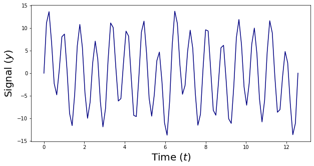
Then again, some indicators have a non-fixed frequency (frequency is certainly time-dependent). Right here’s an instance of this type of sign:
And we will analyze this sign utilizing the chirplet remodel.
In my newest article, I clarify how a chirplet remodel is outlined, the right way to implement it in Python, and the right way to plot it.
One of many questions that I acquired is especially attention-grabbing and it’s the following:
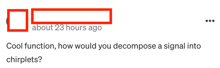
And that is precisely what we’re going to be speaking about on this article 🙃
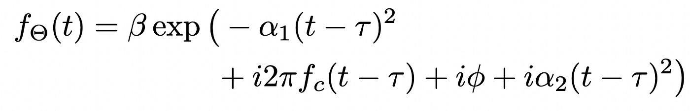
So we all know {that a} Chirplet is a sign with a widely known analytical equation:

And we’ve seen that by altering the set of parameters (beta, alpha1, alpha2, fc, tau and phi) we will describe totally different sorts of chirplets.
Now, let’s say we’ve a brand new chirplet. This chirplet is utterly outlined* by a set of those 6 values.
* By utterly outlined I imply that the sign is represented by one and just one set of parameters and vice-versa.
So let’s say that this sign we wish to characterize by way of a chirplet has the next set of parameters:

How will we get to estimate these 6 parameters?
Let’s say I’m utterly misplaced and I don’t know how to do that process. A quite simple methodology to do this and discover this hat{theta} set of parameters is the so referred to as brute drive. It means:
“Attempt all of the potential mixtures of those 6 parameters and see which one works higher”
This methodology is definitely theoretically doable. After all, if we discretize this 6-dimensional area sufficient, ultimately, we could have a great estimate of the true set of parameters. What’s the drawback although?
Nicely, the true drawback with this methodology is, as at all times after we think about brute drive strategies, the computational complexity.
Let’s say we generate a random chirplet. We do that with the next code:
So that you solely want about (10^-3) seconds to generate a random chirplet. However what number of chirplets do we have to enumerate all of the potential mixtures of chirplets?
Let’s say that k_{variable} is the variety of values of your discrete area. For instance, if all of the alpha_1 values that you’re contemplating are [0,2,5] you’ll have that:

Now, let’s take the next assumptions:

Which means that the variety of chirplets we’ve to think about is the next:

And the computational time is:

Now, let’s change this Okay and see the worth of this computational time.
If we plot this we get fairly an attention-grabbing consequence 😅:
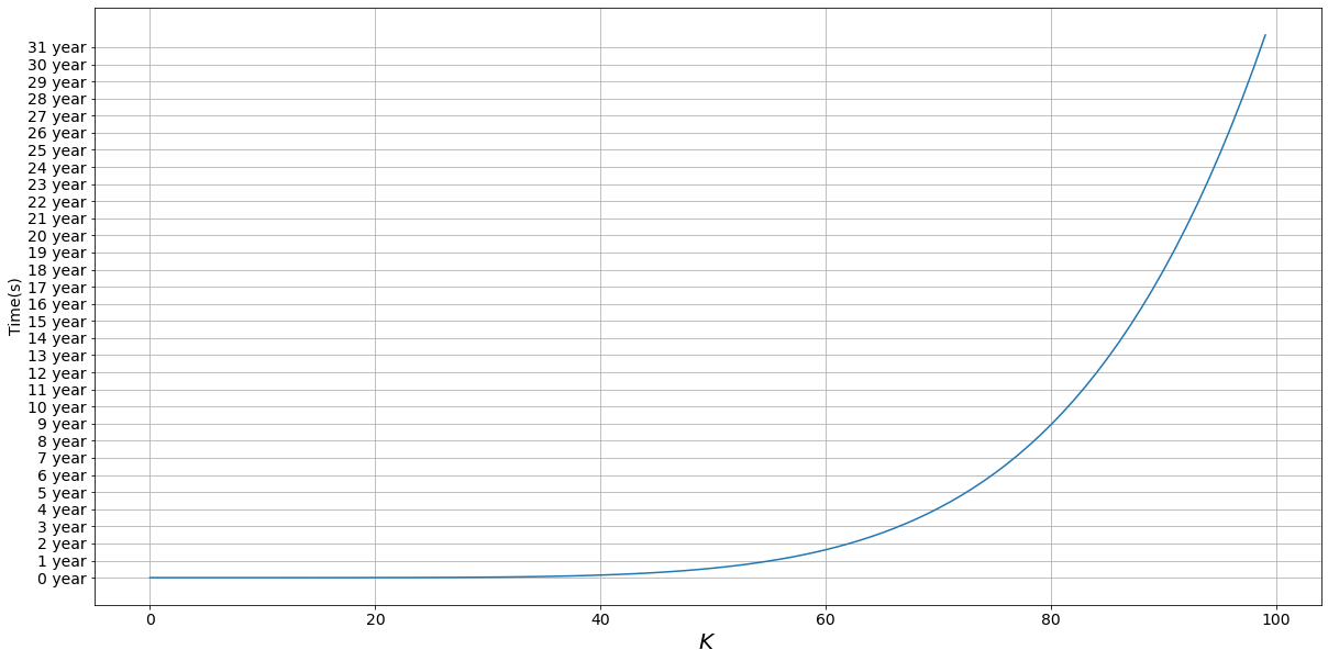
I really feel that whereas we wait 9 years to do our computation for Okay=80 we’d as effectively discover a smarter resolution within the meantime 🙃
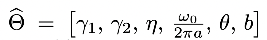
Let’s formalize our aim. Once more, we wish to discover the theta vector:

This theta vector uniquely defines the next chirplet:
Now, after all, we don’t have the analytical expression of this perform, however we solely have its time collection (or numerical illustration).
Now let’s outline a so referred to as chirplet kernel. This chirplet kernel has the next expression.
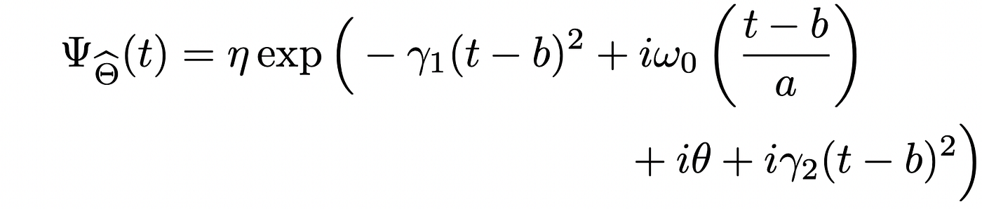
The place:
I feel I’m boring you sufficient so I received’t clarify all the small print of those parameters (however please learn right here if you wish to know them!). The essential factor is that, as you’ll be able to see, the chirplet kernel has the identical expression because the chirplet that we outlined. Now, this chirplet is after all parametric, and it will depend on this hat gamma vector. The thought is then the next:
We challenge our sign on the N-dimensional vector recognized by this chirplet kernel. This projection is parametric and it will depend on the parameters of the chirplet kernel. Then we modify this vector by altering this gamma vector and discovering the optimum worth and getting the correspondent theta (once more, learn right here for extra details about it!)
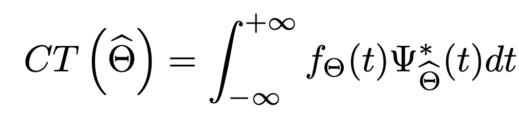
If we wish to discover the largest worth of this projection we compute its gradient. The 0 worth of this gradient will after all give us our optimum worth of hat theta.
Given this formal definition of our drawback, we will now begin discovering our optimum worth. Particularly:
- We iterate over alpha1 discovering the most important coefficient argument
- We iterate over alpha2 discovering the most important coefficient argument
- We discover tau and beta utilizing the Hilbert Remodel
- We discover the frequency (fc) and the part (phi) utilizing the Fourier Remodel
Let’s implement this!
This estimation could be performed with the next code:
Let’s check it!
Utilizing the next perform we estimate the parameters and create our estimated chirplet.
After all, we would like the enter sign to be equivalent to the reconstruction. Let’s see if that’s the case.
Nicely, as we will see the reconstruction is not at all times excellent.
Nonetheless, we noticed that we’re on the lookout for an answer in a big dimensional area (by big I imply that the area grows exponentially with the variety of parameters) and the issue is an NP-hard drawback with a non-unique resolution (learn extra right here).
For these causes, I discover these outcomes fairly nice. 🤩
When you favored the article and also you wish to know extra about Machine Studying, otherwise you simply wish to ask me one thing you’ll be able to:
A. Comply with me on Linkedin, the place I publish all my tales
B. Subscribe to my e-newsletter. It can maintain you up to date about new tales and provide the probability to textual content me to obtain all of the corrections or doubts you’ll have.
C. Change into a referred member, so that you received’t have any “most variety of tales for the month” and you’ll learn no matter I (and hundreds of different Machine Studying and Knowledge Science prime writers) write concerning the latest know-how obtainable.
The paper that has been used as a reference for this text is the next: A Successive Parameter Estimation Algorithm for Chirplet Sign Decomposition. This GitHub folder has additionally been used as a place to begin
