
What makes an remark “uncommon”?

In information science, a standard job is anomaly detection, i.e. understanding whether or not an remark is “uncommon”. Initially, what does it imply to be uncommon? On this article we’re going to examine three alternative ways wherein an remark could be uncommon: it might probably have uncommon traits, it may not match the mannequin effectively or it is perhaps significantly influential in coaching the mannequin. We are going to see that in linear regression the latter attribute is a byproduct of the primary two.
Importantly, being uncommon is not essentially dangerous. Observations which have totally different traits from all others typically carry extra data. We additionally count on some observations to not match the mannequin effectively, in any other case, the mannequin might be biased (we’re overfitting). Nevertheless, “uncommon” observations are additionally extra more likely to be generated by a special data-generating course of. Excessive circumstances embody measurement error or fraud, however different circumstances could be extra nuanced, corresponding to real customers with uncommon traits or behaviors. Area information is at all times king and dropping observations just for statistical causes is rarely sensible.
That stated, let’s take a look at some alternative ways wherein observations could be “uncommon”.
Suppose we had been a peer-to-peer on-line platform and we’re involved in understanding if there’s something suspicious happening with our enterprise. We have now details about how a lot time our customers spend on the platform and the entire worth of their transactions. Are some customers suspicious?
First, let’s take a look on the information. I import the info producing course of dgp_p2p() from src.dgp and a few plotting features and libraries from src.utils. I embody code snippets from Deepnote, a Jupyter-like web-based collaborative pocket book setting. For our objective, Deepnote may be very useful as a result of it permits me not solely to incorporate code but additionally output, like information and tables.
We have now data on 50 customers for which we observe hours spent on the platform and complete transactions quantity. Since we solely have two variables we will simply examine them utilizing a scatterplot.

The connection between hours and transactions appears to observe a transparent linear relationship. If we match a linear mannequin, we observe a very tight match.
Does any information level look suspiciously totally different from the others? How?
The primary metric that we’re going to use to judge “uncommon” observations is the leverage. The target of the leverage is to seize how a lot a single level is totally different with respect to different information factors. These information factors are sometimes known as outliers and there exist an almost infinite quantity of algorithms and guidelines of thumb to flag them. Nevertheless, the concept is identical: flagging observations which might be uncommon by way of options.
The leverage of an remark i is outlined as

One interpretation of the leverage is as a measure of distance the place particular person observations are in contrast in opposition to the common of all observations.
One other interpretation of the leverage is because the affect of the result of remark i, yᵢ, on the corresponding fitted worth ŷᵢ.

Algebraically, the leverage of remark i is the iₜₕ ingredient of the design matrix X’(X’X)⁻¹X. Among the many many properties of the leverages, is the truth that they’re non-negative and their values sum to 1.
Let’s compute the leverage of the observations in our dataset. We additionally flag observations which have uncommon leverages (which we arbitrarily outline as greater than two commonplace deviations away from the common leverage).
Let’s plot the distribution of leverage values in our information.
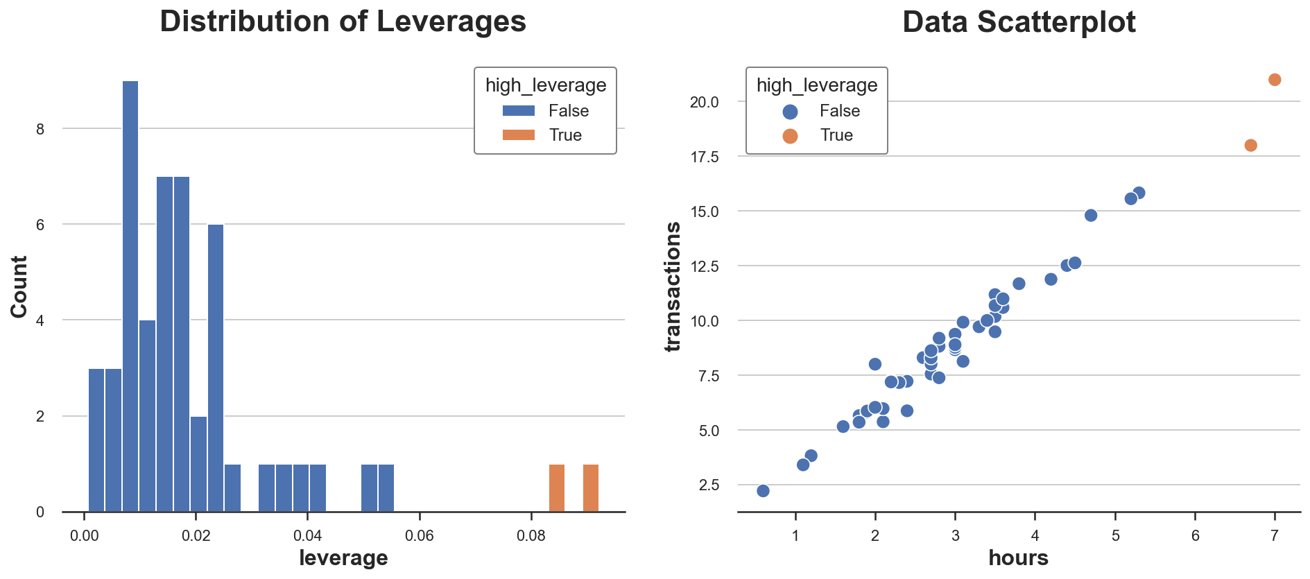
As we will see, the distribution is skewed, with two observations having unusually excessive leverage. Certainly, within the scatterplot, these two observations are barely separated from the remainder of the distribution.
Is that this dangerous information? It relies upon. Outliers are not an issue per se. Really, if they’re real observations, they could carry way more data than different observations. Alternatively, they’re additionally extra possible not to be real observations (e.g. fraud, measurement error, …) or to be inherently totally different from the opposite ones (e.g. skilled customers vs amateurs). In any case, we’d wish to examine additional and use as a lot context-specific data as we will.
One ought to by no means drop observations for statistical causes alone
Importantly, the truth that an remark has a excessive leverage tells us details about the options of the mannequin however nothing in regards to the mannequin itself. Are these customers simply totally different or do in addition they behave in a different way?
To date we have now solely talked about uncommon options, however what about uncommon conduct? That is what regression residuals measure.
Regression residuals are the distinction between the anticipated final result values and the noticed final result values. In a way, they seize what the mannequin can’t clarify: the upper the residual of 1 remark the extra it’s uncommon within the sense that the mannequin can’t clarify it.
Within the case of linear regression, residuals could be written as

In our case, since X is one dimensional (hours), we will simply visualize them as the gap between the observations and the prediction line.

Do some observations have unusually excessive residuals? Let’s plot their distribution.
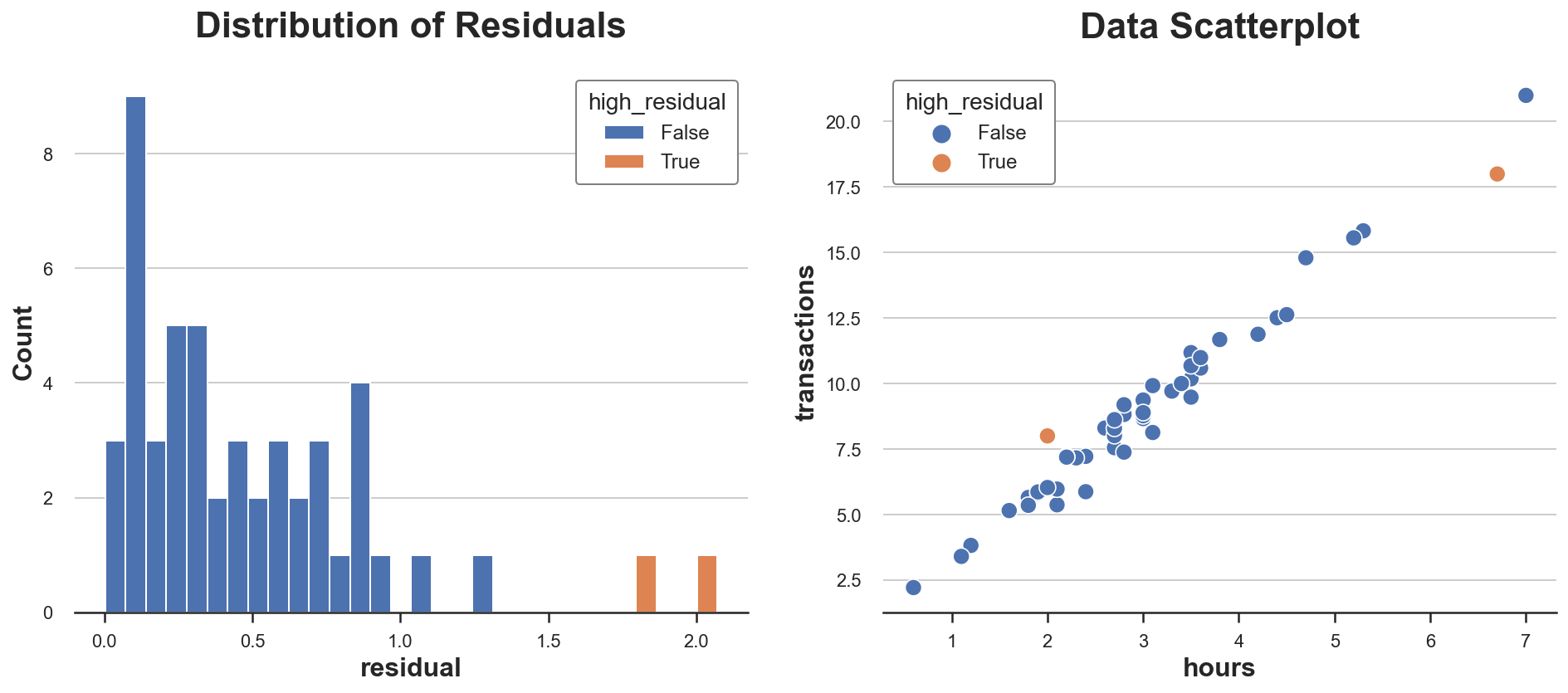
Two observations have significantly excessive residuals. Which means that for these observations, the mannequin just isn’t good at predicting the noticed outcomes.
Is that this dangerous information? Once more, not essentially. A mannequin that matches the observations too effectively is more likely to be biased. Nevertheless, it’d nonetheless be essential to grasp why some customers have a special relationship between hours spent and complete transactions. As standard, area information is essential.
To date we have now checked out observations with “uncommon” traits and “uncommon” mannequin match, however what if the remark itself is distorting the mannequin? How a lot our mannequin is pushed by a handful of observations?
The idea of affect and affect features was developed exactly to reply this query: what are influential observations? This query was highly regarded within the 80s and misplaced attraction for a very long time till lately, due to the rising want of explaining advanced machine studying and AI fashions.
The overall concept is to outline an remark as influential if eradicating it considerably adjustments the estimated mannequin. In linear regression, we outline the affect of remark i as:

The place β̂-i is the OLS coefficient estimated omitting remark i.
As you may see, there’s a tight connection to each the leverage hᵢᵢ and residuals eᵢ: affect is nearly the product of the 2. Certainly, in linear regression, observations with excessive leverage are observations which might be each outliers and have excessive residuals. Not one of the two circumstances alone is adequate for an remark to have an affect on the mannequin.
We will see it greatest within the information.
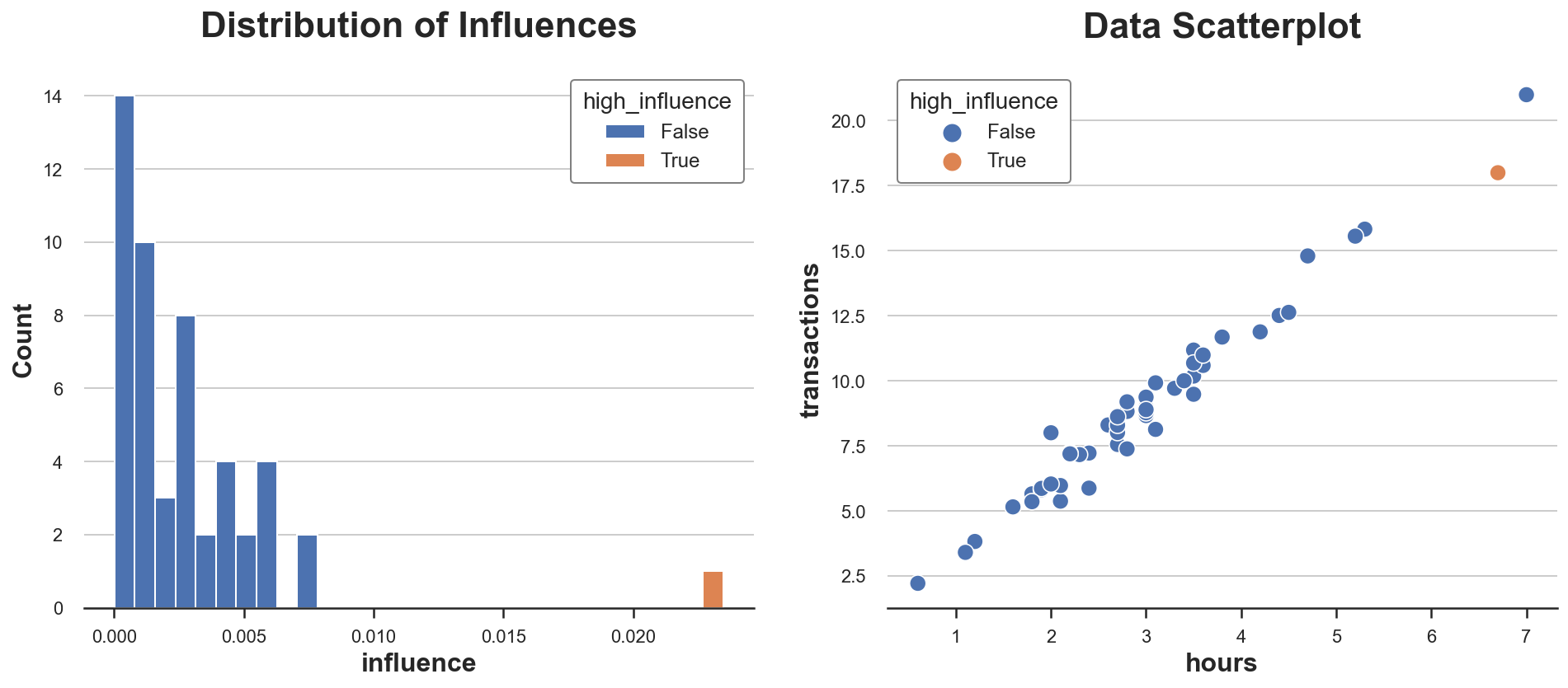
In our dataset, there is just one remark with excessive affect, and its worth is disproportionally bigger than the affect of all different observations. Would you’ve gotten guessed it from the scatterplot alone?
We will now plot all “uncommon” factors in the identical plot. I additionally report residuals and leverage of every level in a separate plot.
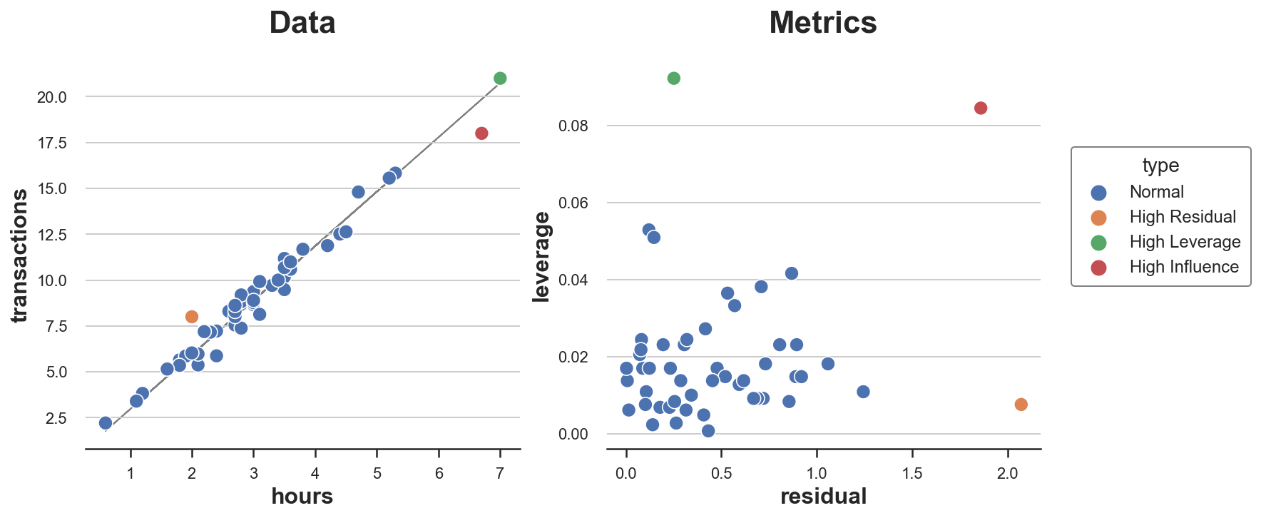
As we will see, we have now one level with excessive residual and low leverage, one with excessive leverage and low residual, and just one level with each excessive leverage and excessive residual: the one influential level.
From the plot, it’s also clear why not one of the two circumstances alone is adequate for an remark to be influential and warp the mannequin. The orange level has a excessive residual but it surely lies proper in the midst of the distribution and subsequently can’t tilt the road of greatest match. The inexperienced level as a substitute has excessive leverage and lies removed from the middle of the distribution but it surely’s completely aligned with the road of match. Eradicating it might not change something. The pink dot as a substitute is totally different from the others by way of each traits and conduct and subsequently tilts the match line in direction of itself.
On this submit, we have now seen a few alternative ways wherein observations could be “uncommon”: they’ll have both uncommon traits or uncommon conduct. In linear regression, when an remark has each it’s also influential: it tilts the mannequin in direction of itself.
Within the instance of the article, we targeting a univariate linear regression. Nevertheless, analysis on affect features has lately change into a scorching subject due to the necessity to make black-box machine studying algorithms comprehensible. With fashions with hundreds of thousands of parameters, billions of observations, and wild non-linearities, it may be very laborious to determine whether or not a single remark is influential and the way.
References
[1] D. Prepare dinner, Detection of Influential Statement in Linear Regression (1980), Technometrics.
[2] D. Prepare dinner, S. Weisberg, Characterizations of an Empirical Affect Perform for Detecting Influential Circumstances in Regression (1980), Technometrics.
[2] P. W. Koh, P. Liang, Understanding Black-box Predictions through Affect Features (2017), ICML Proceedings.
Code
You’ll find the unique Jupyter Pocket book right here:
Thanks for studying!
I actually admire it! 🤗 When you preferred the submit and want to see extra, take into account following me. I submit as soon as every week on matters associated to causal inference and information evaluation. I attempt to preserve my posts easy however exact, at all times offering code, examples, and simulations.
Additionally, a small disclaimer: I write to study so errors are the norm, though I attempt my greatest. Please, if you spot them, let me know. I additionally admire options on new matters!
