I used to be personally ineffective for many of the Spring of 2020. There was a time period, although, after the height in coronavirus circumstances right here in NYC and earlier than the onslaught of police violence right here in NYC that I managed to scrounge up the motivation to do one thing apart from drink and maniacally refresh my Twitter feed. I got down to work on one thing fully meaningless. It was nearly therapeutic to work on a challenge with no worth of any variety (insert PhD joke right here).
A aspect impact of getting spent 10 years with restricted revenue in school and grad college, 6 of these right here in costly ass NYC, is that I eat of lot of low-cost sandwiches, regardless that I now have a pleasant Tech™ job. Whereas my sandwich consumption was fairly formidable pre-covid, sheltering in place cemented this staple in my weight loss program. I’m notably keen on peanut butter and banana sandwiches, having been launched to them as a baby by my maternal grandfather who ate them often.
I begin a peanut butter and banana sandwich by spreading peanut butter on two slices of bread. I then slice round slices of the banana, beginning on the finish of the banana, and place every slice on one of many items of bread till I’ve a single layer of banana slices. Each time I do that, the previous condensed matter physicist in me begins to twitch his eye. You see, I’ve this urge, this need, this want to maximise the packing fraction of the banana slices. That’s, I need to maximize the protection of the banana slices on the bread. Simply as bowl-form meals is ideal since you get each ingredient in each chunk, every chunk of my sandwich ought to yield the identical golden ratio of bread, peanut butter, and banana.
Should you had been a machine studying mannequin (or my spouse), then you definitely would inform me to only minimize lengthy rectangular strips alongside the lengthy axis of the banana, however I’m not a sociopath. If life had been easy, then the banana slices could be good circles of equal diameter, and we might coast alongside trying up optimum configurations on packomania. However alas, life is just not easy. We’re in the course of a world pandemic, and banana slices are elliptical with various measurement.
So, how can we make optimum peanut butter and banana sandwiches? It’s actually fairly easy. You are taking an image of your banana and bread, go the picture by way of a deep studying mannequin to find mentioned gadgets, do some nonlinear curve becoming to the banana, remodel to polar coordinates and “slice” the banana alongside the fitted curve, flip these slices into elliptical polygons, and feed the polygons and bread “field” right into a 2D nesting algorithm.
You will have seen that I supposedly began this challenge within the Spring, and it’s now August. Like most fool engineers, I had no concept how difficult this silly challenge was going to be, however time’s meaningless in quarantine, so right here we’re. And right here you might be! As a result of I made a pip installable python bundle nannernest if you wish to optimize your personal sandwiches, and I’m going to spend the remainder of this publish describing how this entire godforsaken factor works.
Sandwich Segmentation
I do know that deep studying has been correctly commoditized when the simplest a part of this challenge was figuring out each pixel that belongs to a banana or slice of bread in a picture. Significantly, this step was tremendous simple. I used a pretrained Masks-RCNN torchvision mannequin with a Resnet spine. The mannequin was pretrained on the COCO dataset, and fortunately the dataset has “banana” as segmentation class, together with “sandwich” and “cake” which had been shut sufficient classes for appropriate detection of most slices of bread.
Passing a picture by way of the mannequin outputs a bunch of detected objects, the place every detected object has an related label, rating, bounding field, and masks, the place the masks identifies the pixels that correspond to the thing with a weight at every pixel equivalent to the mannequin’s confidence in that pixel’s label.
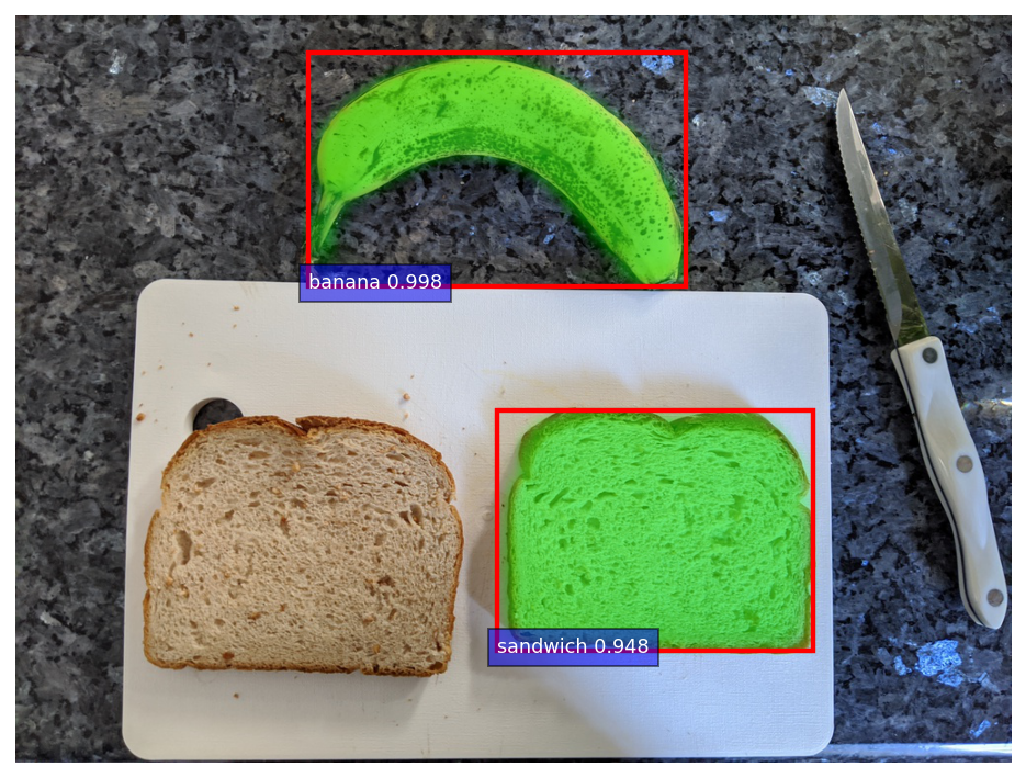
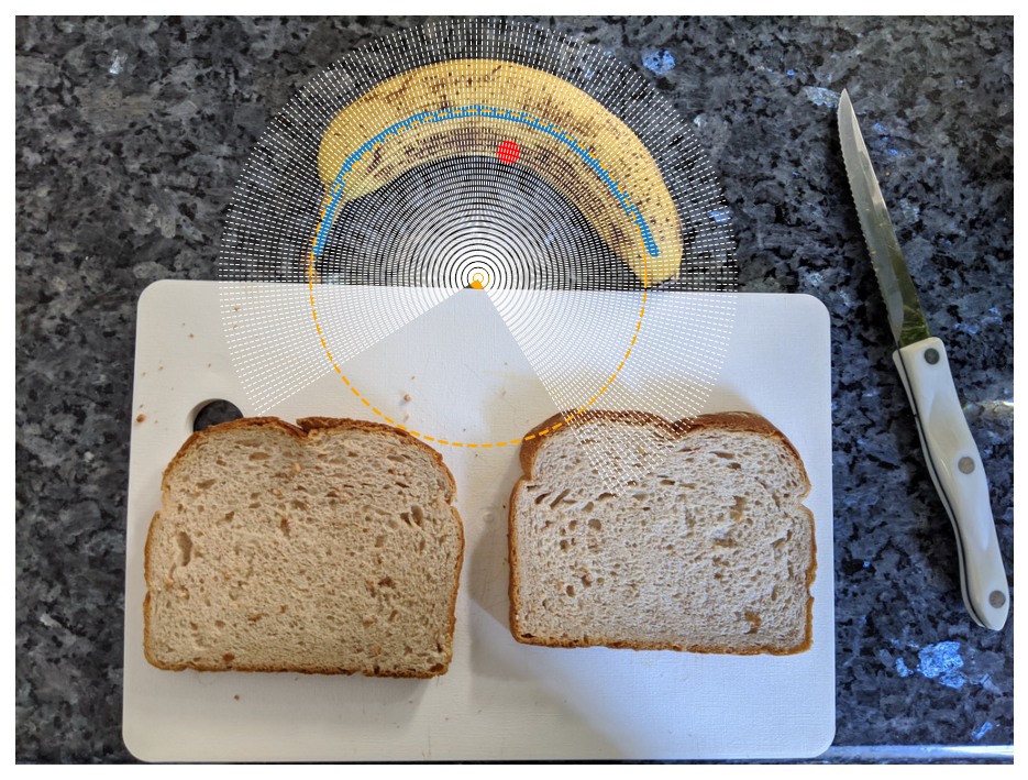
As a result of there may very well be a number of bananas and slices of bread within the picture, I pick the banana and slice of bread with the very best rating. Under, you possibly can see the mannequin is clearly in a position to establish the banana and bread, with the masks overlaid in a semi-transparent, radioactive inexperienced.
%config InlineBackend.figure_format = 'retina'

from pathlib import Path
import matplotlib.pyplot as plt
import numpy as np
import nannernest

_RC_PARAMS = {
    "determine.figsize": (8, 4),
    "axes.labelsize": 16,
    "axes.titlesize": 18,
    "axes.spines.proper": False,
    "axes.spines.prime": False,
    "font.measurement": 14,
    "strains.linewidth": 2,
    "strains.markersize": 6,
    "legend.fontsize": 14,
}
for okay, v in _RC_PARAMS.gadgets():
    plt.rcParams[k] = v

DPI = 160
picture, banana, bread = nannernest.segmentation.run(Path("pre_sandwich.jpg"))
nannernest.viz.plot(picture, banana=banana, bread=bread, present=True, dpi=DPI)
Now that we now have recognized the banana within the picture, we have to just about “slice” it. That is the place we’re first launched to the common ache of laptop imaginative and prescient:
By eye, I can see precisely what I need to do; by code, it’s so rattling troublesome.
I might ask you to attract strains on the banana figuring out the place you’d slice it, and you would simply draw well-spaced, considerably parallel slices. It’s not really easy to do that with code. Nevertheless, I might additionally argue that that is the enjoyable a part of the issue. There are a lot of methods to resolve this, and it feels artistic, versus utilizing a pre-trained deep studying mannequin. Then again, “creatively” fixing these issues possible results in extra brittle options in comparison with deep studying fashions skilled on hundreds of thousands of examples. There’s a tradeoff right here.
I attempted a bunch of analytical options primarily based on ellipses, however nothing appeared to work fairly proper. I ended up touchdown on a considerably easier resolution that will not be strong to straight bananas, however who cares – this can be a foolish challenge anyway. Utilizing the great scikit-image library, I first calculate the skeleton of the banana segmentation masks. This reduces the masks to a one pixel extensive illustration which successfully creates a curve that runs alongside the lengthy axis of the banana.
slices, banana_circle, banana_centroid, banana_skeleton = nannernest.slicing.run(
    banana.masks
)
nannernest.viz.plot(picture, banana_skeleton=banana_skeleton, present=True, dpi=DPI)
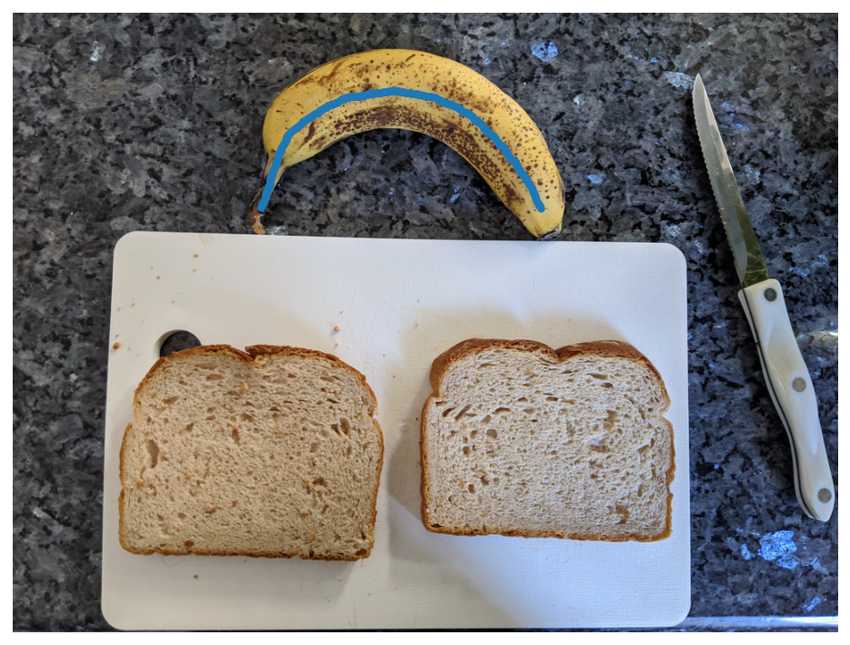
I then match a circle to the banana skeleton utilizing a pleasant scipy-based least squares optimization I discovered right here. I really initially tried to suit this with PyTorch and completely failed, possible attributable to the truth that that is really a nonlinear optimization downside.
nannernest.viz.plot(
    picture,
    banana_skeleton=banana_skeleton,
    banana_circle=banana_circle,
    present=True,
    dpi=DPI,
)

Rad Coordinate Transformations
With the circle match to the banana, the purpose is to now draw radial strains out from the middle of the circle to the banana and have every radial line correspond to the slice of a knife. Once more, whereas it’s simple to visualise this, it’s a lot tougher in apply. For instance, we have to begin slicing at one finish of the banana, however how do we discover an finish of the banana? Additionally, there are two ends, and we now have to distinguish between them. Opposite to the habits of monkeys, I begin slicing my bananas on the stem finish, and that’s what we’re going to do right here.
Crucially, as a result of we now have this circle and need to minimize radial slices, we should remodel from cartesian to polar coordinates and orient ourselves each radially and angularly with respect to the banana. As a begin for orienting ourselves angularly, we calculate the centroid of the banana masks, which corresponds to the middle of mass of the banana masks if the banana masks had been a 2D object. The centroid is proven beneath as a crimson dot.
We now draw a radial line originating from the banana circle and passing by way of the centroid, proven because the dashed white line beneath. We’ll contemplate that line to mark our reference angle which orients us to the middle of the banana.
ax = nannernest.viz.plot(
    picture,
    banana_skeleton=banana_skeleton,
    banana_circle=banana_circle,
    banana_centroid=banana_centroid,
    present=False,
    dpi=DPI,
)

dy = banana_centroid[0] - banana_circle.yc
dx = banana_centroid[1] - banana_circle.xc
reference_angle = np.arctan2(dy, dx)
radius = np.sqrt(dx ** 2 + dy ** 2)

radial_end_point = (
    banana_circle.xc + 2 * radius * np.cos(reference_angle),
    banana_circle.yc + 2 * radius * np.sin(reference_angle),
)

ax.plot(
    (banana_circle.xc, radial_end_point[0]),
    (banana_circle.yc, radial_end_point[1]),
    colour="white",
    linestyle="--",
    linewidth=1,
)
None

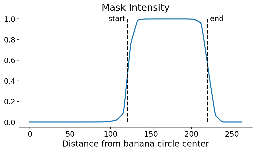
Utilizing scikit-image, we calculate the segmentation masks depth alongside this radial line utilizing the profile_line operate. As a result of our line is passing at an angle alongside discrete masks pixels (aka matrix entries), we take a mean of neighboring factors alongside the radial line minimize utilizing the linewidth arguments. As you possibly can see, the banana masks pops out just a little over 100 factors from the banana circle heart.
from skimage import measure

profile_line = measure.profile_line(
    banana.masks.T, banana_circle.heart, radial_end_point, linewidth=2, mode="fixed"
)
fig, ax = plt.subplots()
ax.plot(profile_line)
ax.set_xlabel("Distance from banana circle heart")
ax.set_title("Masks Depth")
None
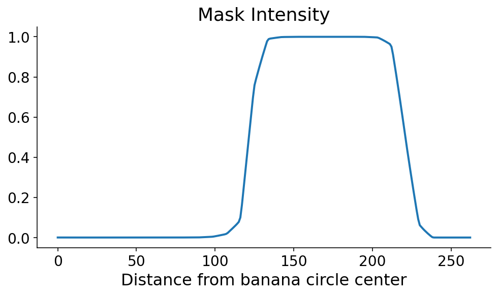
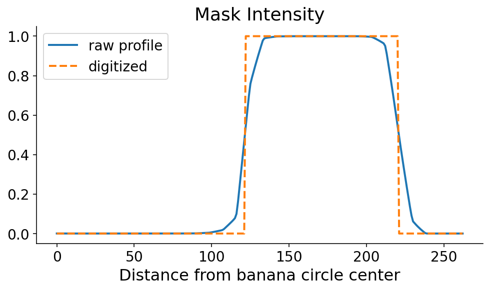
This profile line is what permits us to orient ourselves radially. You’ll be able to clearly see the place the banana begins and ends, within the radial path. As at all times, simply seeing it isn’t adequate. We’d like code to outline the beginning and finish of the banana on this path. The masks tends to be monotonically growing after which monotonically reducing alongside the beginning and finish, respectively. Utilizing this info, there are a pair ways in which we might outline the beginning and the top. If the steepest components of the profile line happen initially and finish, then the beginning and finish would correspond to the utmost and minimal derivatives, respectively. I’m just a little nervous about noise within the masks sign when the mannequin confidence is low, so I first digitize (or threshold) the profile line by setting it to 0 (1) if it’s lower than (higher than) 0.5.
digitized = profile_line > 0.5

fig, ax = plt.subplots()
ax.plot(profile_line, label="uncooked profile")
ax.plot(digitized, "--", label="digitized")
ax.legend()
ax.set_xlabel("Distance from banana circle heart")
ax.set_title("Masks Depth")
None
We now seek for the factors the place the sign flips by way of the maxmimum and minimal derivatives of the digitized sign. This may be achieved with some fast numpy. It’s nonetheless a harmful (quote: “harmful”, it’s a banana) operation which might amplify noise. One choice sooner or later could be to clean the profile line previous to taking the by-product.
diff = np.diff(digitized, append=0)
begin, finish = np.argmax(diff), np.argmin(diff)
fig, ax = plt.subplots()
ax.plot(profile_line)
ax.plot((begin, begin), (0, 1), "k--")
ax.plot((finish, finish), (0, 1), "k--")
ax.annotate("begin ", (begin, 1), ha="proper", va="heart")
ax.annotate(" finish", (finish, 1), ha="left", va="heart")
ax.set_xlabel("Distance from banana circle heart")
ax.set_title("Masks Depth")
None
$phi$-House
We are actually in a position to orient ourselves angularly with respect to the middle of the banana and radially by way of the beginning and finish of the banana alongside the radial line. The final step is the discover the angular begin and finish of the banana, the place the angular begin will correspond to the angle pointing to the stem of the banana. To that finish, we begin by creating an array of angles which span from the reference centroid angle minus 135$^{circ}$ to the reference angle plus 135$^{circ}$. Analogous to numpy’s linspace, we’ll name this array $phi$-space.
For every angle in $phi$-space, we’ll calculate a profile line like we did above. Under, we create a $phi$-space of 201 factors and draw every of those profile strains on the unique picture. You’ll be able to see that they clearly cowl the banana with some wholesome room on both angular aspect.
phi_space = nannernest.slicing.create_phi_space(
    banana_centroid, banana_circle, num_points=201
)
profiles = nannernest.slicing.assemble_profiles(
    phi_space, banana.masks, banana_circle, linewidth=2
)
ax = nannernest.viz.plot(
    picture,
    banana_skeleton=banana_skeleton,
    banana_circle=banana_circle,
    banana_centroid=banana_centroid,
    present=False,
    dpi=DPI,
)
for phi in phi_space:
    radial_end_point = (
        banana_circle.xc + 2 * radius * np.cos(phi),
        banana_circle.yc + 2 * radius * np.sin(phi),
    )
    ax.plot(
        (banana_circle.xc, radial_end_point[0]),
        (banana_circle.yc, radial_end_point[1]),
        colour="white",
        linestyle="--",
        linewidth=0.5,
    )
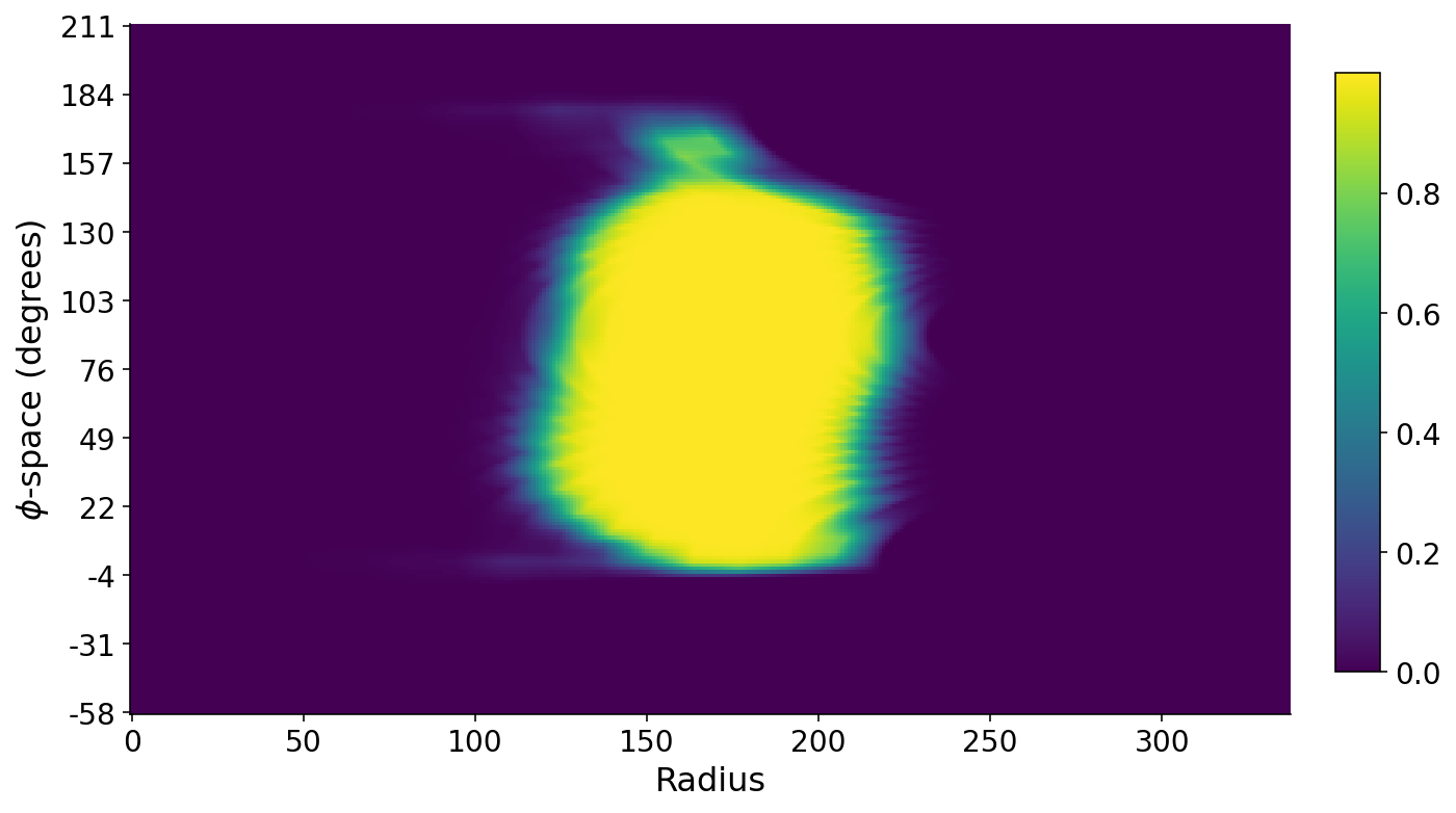
We are able to additionally stack all the profile strains on one another such that we now have a matrix the place the rows are angles, the columns denote radial distance, and the values are the masks intensities alongside these strains. A false-color plot of this matrix beneath exhibits the banana. The lengthy axis of the banana roughly runs alongside the $phi$-space path. The small little bit of banana on the prime corresponds to the banana stem. The $phi$-space angles are with respect to the horizontal axis.
fig, ax = plt.subplots(figsize=(10, 10))
im = ax.imshow(profiles)

ax.set_xlabel("Radius")
ax.set_ylabel("$phi$-space (levels)")
ticks = np.linspace(0, len(phi_space) - 1, 11, dtype=np.int32)

ax.set_yticks(ticks)
ax.set_yticklabels((phi_space[ticks] * 180 / np.pi).astype(int))

plt.colorbar(im, cax=fig.add_axes([0.93, 0.3, 0.03, 0.4]))
None
Slicing from Stem to Seed
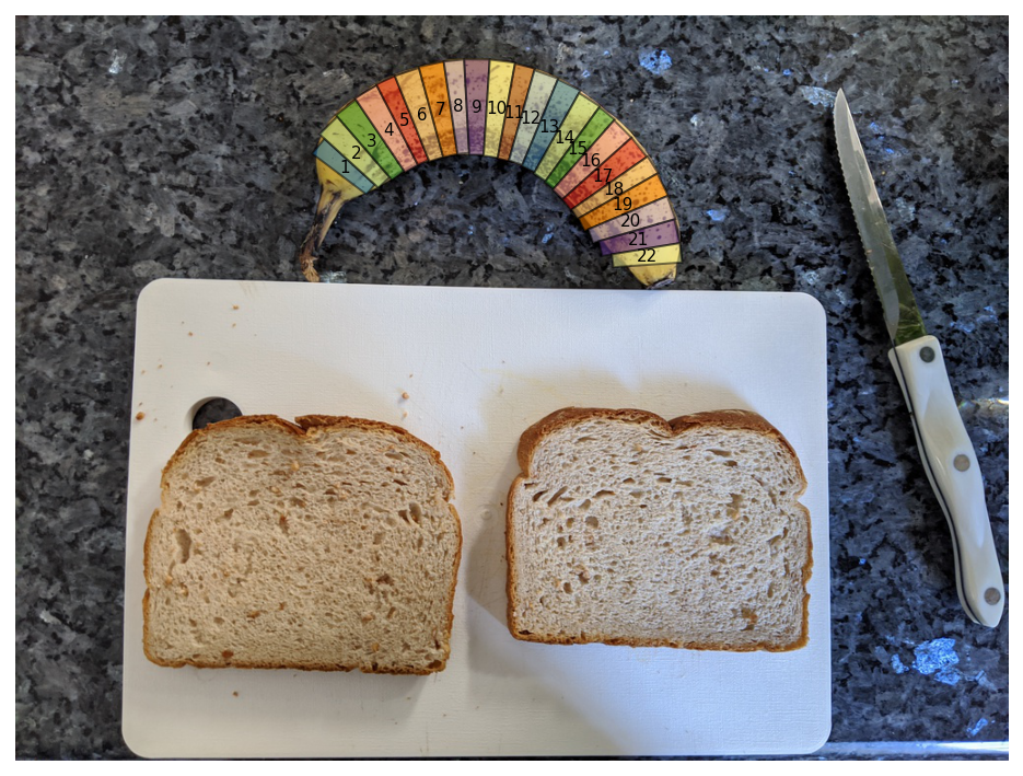
Lastly, with this odd matrix above that represents this polar world warped onto a cartesian plot, we are able to establish each the banana stem and the alternative finish of the banana which homes its seed. I discover the 2 ends of the banana utilizing an analogous technique to earlier for locating the radial begin and finish of the banana. I then discover the common masks depth in a area round both finish of the banana and assume that the stem has a smaller common depth. Lastly, I just about “chop off” the stem utilizing the data that the seed aspect of the banana ought to have related common depth to the stem aspect sans stem.
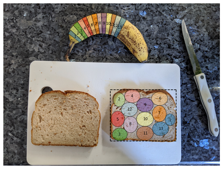
With this work achieved, I’ve now recognized the angular place of the stem and seed of the banana, together with the radial begin and finish of the banana at any angle. I slice the banana by chopping it up into evenly spaced angles and drawing an oblong slice at every angle spacing. I go away as a free parameter the entire variety of slices which implicitly determines the banana slice thickness. By default, I slice 23 slices and throw out the primary and final slice (no one desires these).
nannernest.viz.plot(picture, slices=slices, present=True, dpi=DPI)
Ellipsoidal Assumptions
We now need to make two assumptions in regards to the banana slices. Firstly, we all know that the banana slices will likely be smaller than those proven above as a result of the peel has finite thickness. Secondly, bananas should not completely round, and the slices will come out as ellipses. Based mostly on a pair poor measurements with a tape measure (I don’t have calipers), I assume that the precise banana slices are 20% smaller than the picture above with the banana peel. I additionally take the slices within the picture above to characterize the most important axis of the banana slice ellipse, and assume that the minor axis is 85% the dimensions of the most important axis.
With these assumptions in place, slice 1 proven above seems like
fig, ax = plt.subplots(figsize=(8, 8))
theta = np.linspace(0, 2 * np.pi, 101)
ax.plot(
    (slices[0].major_axis / 2) * np.cos(theta),
    (slices[0].minor_axis / 2) * np.sin(theta),
)
lim = slices[0].major_axis / 2 + 1
ax.set_xlim((-lim, lim))
ax.set_ylim((-lim, lim))
None
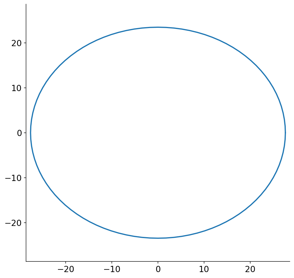
Previous to the ultimate step of this ridiculously lengthy pipeline, we now have to transform the ellipsoidal slices into polygons. Technically, the plot above is a discrete set of factors and may very well be thought of a polygon. To make the issue tractable, although, we cut back the ellipse to a small set of factors. After I first began engaged on this downside, I didn’t know if I used to be going to be severely restricted in what number of factors I might allot for every slice polygon. I’m additionally considerably neurotic (a light understatement) and apprehensive about the truth that the polygon will essentially not be the very same measurement because the ellipse.
To resolve this, I wished to determine the polygon that circumscribes the ellipse. I used to be stunned to not discover any code for this, so I ended up attempting to resolve it analytically. The ensuing algebra was fairly gnarly, so there’s now a operate in nannernest that runs sympy and calculates the scaling elements for the most important and minor axes primarily based on the variety of factors within the ellipse polygon.
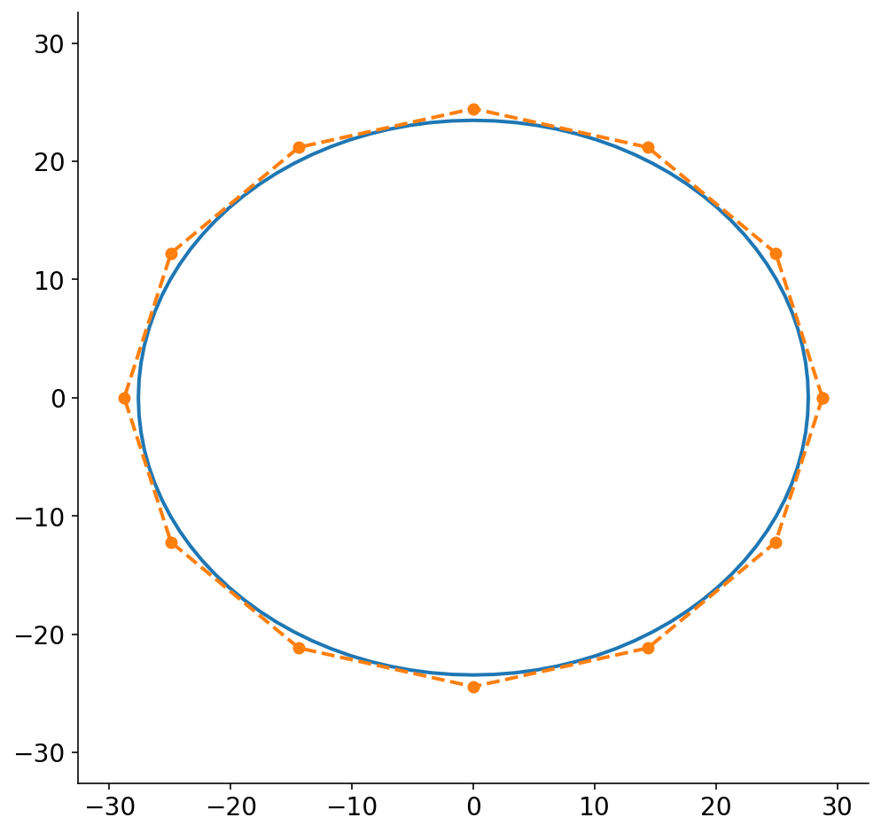
Under, I draw the ellipse and the circumscribed polygon for a polygon of 12 factors. Whereas (by definition) the circumscribed polygon is larger than the ellipse, the distinction is kind of small. I most likely might have simply chopped the unique ellipse into 12 factors with out a lot loss in accuracy. In apply, I’ve been utilizing 30 factors which solely makes the distinction even smaller. Additionally, FWIW, I feel that my algebra solely works if there are polygon factors instantly alongside the x and y axes, so there you go. If anyone has a closed type resolution to this, I’d like to see it!
fig, ax = plt.subplots(figsize=(8, 8))
theta = np.linspace(0, 2 * np.pi, 101)
slice_x = (slices[0].major_axis / 2) * np.cos(theta)
slice_y = (slices[0].minor_axis / 2) * np.sin(theta)
ax.plot(slice_x, slice_y)
lim = max(slice_x.max(), slice_y.max()) + 5

num_points = 12
major_scaler, minor_scaler = nannernest.nesting.calc_elliptical_polygon_scalers(
    num_points
)
poly = nannernest.nesting.ellipse_to_polygon(
    slices[0], num_points, major_scaler, minor_scaler
)
ax.plot(*zip(*poly), "o--")

ax.set_xlim((-lim, lim))
ax.set_ylim((-lim, lim))
None
Bread Field
This half was fairly fast. I wanted to outline the bread as a “field” inside which to nest my banana slices. Initially, I simply used the bounding field from the segmentation algorithm. Nevertheless, the bounding field simply defines the utmost boundary of the bread. On a whim, I attempted rotating a picture by 30$^{circ}$ (sorry, I carried out “information augmentation”), and I discovered that the bounding field didn’t rotate with the bread. Fortunately, I had the segmentation masks, and I grabbed a rotating calipers python implementation to search out the minimal space bounding field that comprises the masks.
Slices in a Nest
By the point I lastly received to the purpose of getting polygonal, ellipsoidal banana slices extracted from a picture and a pleasant bread field, I assumed I might be dwelling free. Absolutely, there’s a easy algorithm that I can plug the polygons and field into to maximise protection? It seems that such a downside generally known as “nesting” or “packing” is extraordinarily onerous. Like, NP-hard. Surprisingly, this can be a in style analysis areas as a result of there are a complete bunch of purposes. Shut packing polygons is analogous to attempting to make use of probably the most materials when slicing a sheet of steel with a CNC machine or slicing out clothes patterns from cloth. I even noticed that an utility of nesting ellipses includes injecting dye into the mind for imaging. The dye spreads out as an ellipse, and one desires most protection with the fewest variety of injections.
I initially got down to discover an analytical resolution to packing ellipses in a field, however this doesn’t appear to actually exist. As time went on, I settled for any respectable resolution to nesting polygons in a field. The favored options are inclined to contain putting polygons one by one within the field. Every polygon touches the earlier polygon. One typically begins at a nook of the field, and fills it up row by row. This sounds easy, however it’s important to construct up a bunch of code to the touch two polygons with out them overlapping. The polygons will also be rotated, positioned in no matter order you need, and so forth… The combinatorial search house is huge, so individuals typically make use of the next optimizations
- Discover a fast technique to find out all the potential factors at which two polygons can contact. That is achieved by way of the No-fit polygon
- Cache the outcomes of 1.
- Select the order of your polygons in a sensible manner, like greatest first.
- Outline an general goal after which make use of a black field optimizer to go looking the house extra effectively. The house includes issues like order of polygon placement and the angle of the polygon when it’s positioned.
For months, I waffled backwards and forwards between looking out GitHub for implementations and attempting to code up my very own. One night time I might spend 3 hours failing to compile C dependencies, whereas the following night time I might learn tutorial papers and hack away. Ultimately, I received about midway to an answer earlier than stumbling upon nest2D which supplies python bindings for a C++ library. Determining this library’s C dependencies wasn’t too dangerous. The one output of the library is an SVG file with a hard and fast rectangular form containing pictures of the nested polygons, so I’ve to parse the SVG afterwards, scale the polygons again to their unique picture, then translate and rotate them to overlay with the unique bread field. Nonetheless, this all ended up being simpler than ending my very own library.
Fortunately, the nesting library is kind of quick, so I begin with 2 banana slices and preserve operating the nesting algorithm with an increasing number of slices till no extra may be added.
And in the long run, we lastly get the banana slices nested within the bread field.
slices, bread_box = nannernest.nesting.run(slices, bread)
nannernest.viz.plot(picture, slices=slices, bread_box=bread_box, present=True, dpi=DPI)
nannernest
As talked about initially, I constructed a bundle known as nannernest so that you can make your personal optimum peanut butter and banana sandwiches. When you get the bundle put in, you possibly can generate your personal optimum sandwiches on the command line with:
$ nannernest pic_of_my_bread_and_banana.jpg
A pair random reflections on constructing this bundle:
- It’s troublesome to transition between completely different “reference frames” when doing laptop imaginative and prescient. Photos are matrices, and their x-direction when plotted corresponds to columns, that are the second index of the matrix. Conversely, we frequently take care of factors or units of factors the place the primary index coresponds to the x path. This will get complicated. I typically needed to convert between cartesian and polar coordinates and place an object within the bigger picture. Retaining monitor of your coordinate methods and scaling elements may be troublesome, and it’s most likely price doing this in a sensible manner. I didn’t actually try this.
- Typer is fairly nice for constructing command line purposes.
- poetry makes bundle growth much less painful.
- dataclasses are an excellent purpose to improve to Python 3.7.
- There are a lot of, many enhancements that may very well be made. The bundle is just not strong and fails in bizarre methods. Slices typically find yourself off the nook of the bread attributable to me utilizing a bounding field to outline the bread quite than the precise define of the bread. I shudder to think about the adversarial assaults that this poor bundle will obtain (assume sizzling canine/not sizzling canine…).
An Optimum Peanut Butter and Banana Sandwich
Currently, my desire is
Better of luck together with your sandwich making. I want you optimum protection.


