Find out about your clients’ ordering habits and select one of the best technique for rising the worth of your orders
These metrics may also help you in understanding how your clients buy at an “order stage”. Completely different dimensions, comparable to your product portfolio’s worth vary, acquisition channel, and placement, can have an effect on these metrics. You can even use them as a comparability to different industries.
The thought is to achieve a very good understanding of your clients’ buy habits earlier than making an attempt new promoting methods to extend order worth.
Let’s begin with an instance, suppose you promote the next objects:
- A t-shirt (15€)
- A hoodie (35€)
- A solar hat (10€)
You observe that your common order worth (AOV) is 13,75€. This may imply that your clients buy a few objects per order and in addition low-value merchandise.
To be extra exact, we must have a look at our orders’ worth distribution and use extra metrics comparable to median or mode, or normal deviation to present a broader image than simply the common order worth.
Utilizing extra dimensions
You possibly can additionally have a look at these metrics (common, median, mode) on your order’s worth damaged down by nation or acquisition channel, and many others…
The objective can be to identify a special habits or totally different developments. Possibly clients acquired by electronic mail channels are utilizing extra reductions (leading to a decrease order worth), versus clients in France who’re liking your product and due to this fact order extra portions or mix a number of objects per order (leading to a higher order worth).
Utilizing benchmarks
Benchmarks can be utilized to check your organization’s efficiency towards others. If benchmarks within the style business present an AOV of 60€ and you’ve got a 13,75€ AOV, maybe your gross sales technique is probably not as efficient.
Nevertheless, understand that your common order worth is depending on a number of features comparable to your pricing level, area/location, market section, and so forth…
One instance of an internet site that gives AOV benchmarks for various industries.
Methods for rising order values
As we focus right here on SQL, I’d advocate studying about what methods you should utilize to extend your common order worth in these totally different articles.
Let’s outline our three metrics and clarify what gross sales knowledge we will probably be utilizing.
- Common: It’s the complete quantity spent by a buyer on an order, averaged throughout all orders. It might probably inform you how a lot you’ll be able to count on a buyer to spend on an order.
- Median: It’s the center worth throughout all of your orders. Because of this 50% of your orders have a price smaller or equal to the median and 50% of your orders have a price increased or equal to the median.
- Mode: It’s probably the most frequent worth throughout all orders. Possibly you have got a star-selling product, and plenty of of your clients are making the identical order.
To compute these metrics, we’re utilizing gross sales knowledge from the official Google Merchandise store, and our desk has for every row, a product, a amount, a income, and the related order id. We’ll name this desk our “base desk”.

Computing the worth of every order
Our first step is to get a price for every order. In our case, the column product income already takes into consideration the amount bought. Because of this we simply must sum the product income per Order ID to get the order worth.
This may return merely for every order, how a lot income is generated (our order worth) in euros.

In our case, we now have round 11k orders, every one having a price (income in euro €).
Orders worth histogram
The median, imply, and common are simpler to interpret after we know the place they sit in our total datasets. A histogram can be utilized for example this.
This may result in the next chart in Datastudio, which is able to assist us perceive higher how our clients are buying.
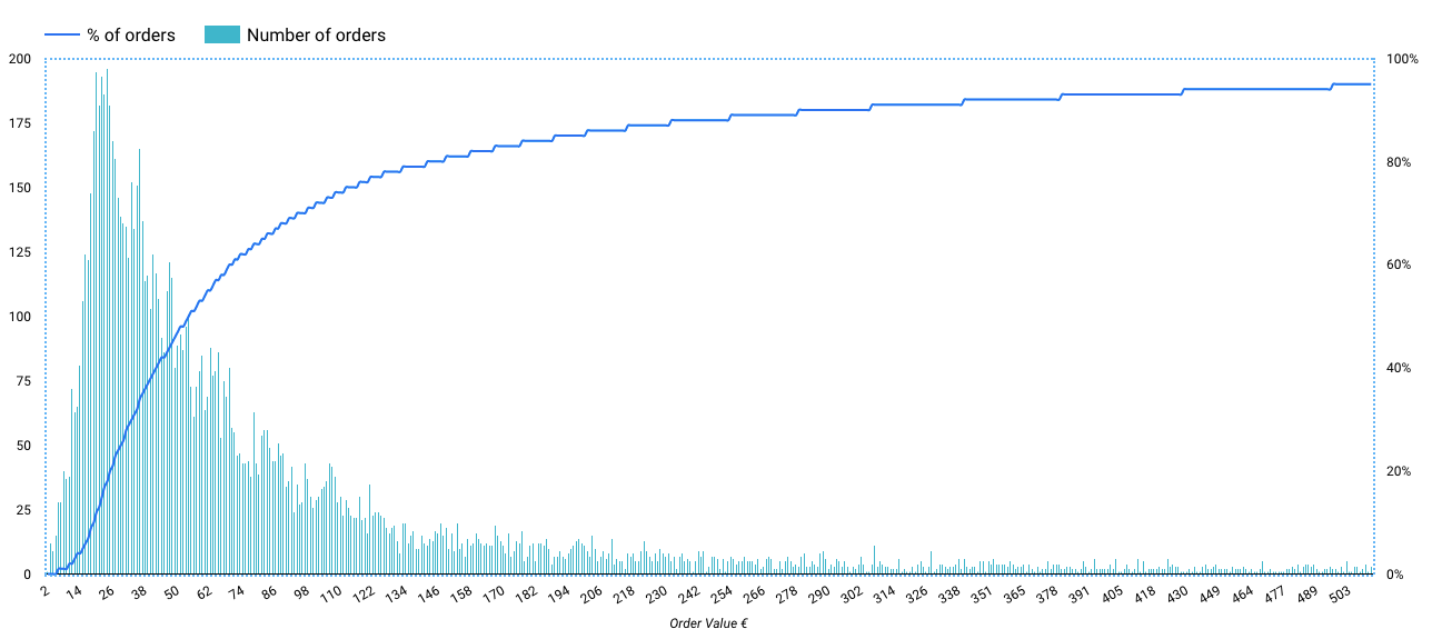
The sunshine blue bars are displaying the distribution of the worth for every of our orders. We will observe that most of our orders are between 15–50 euros and that we now have a very lengthy tail of orders which are greater than 100 euros.
The sturdy blue line exhibits us what number of orders are represented in comparison with the whole of orders (11k in our case). We see right here that 80% of our orders have a price between 0 and 140 euros. That is useful to know if you see a protracted tail of order.
We aren’t reaching 100% on the precise axis of our graph, as a result of we’re not plotting all the info factors. Some orders are generated an enormous quantity of income (we do have orders going from 2 euros to 47 000 euros), which is perhaps thought of outliers.
We may use buckets to higher plot the whole datasets behind and see methods to take away outliers.
In our case, we are going to take away all orders which are higher than 690 euros because it represents solely 3% of our orders.
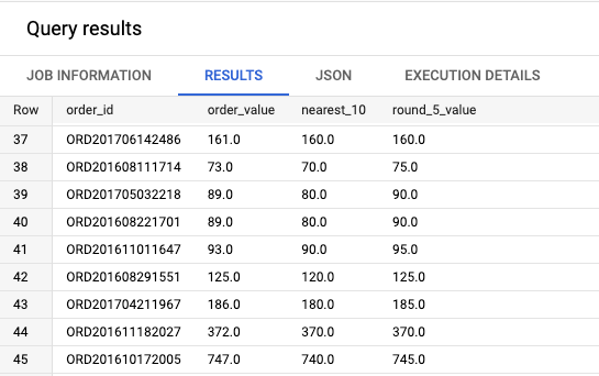
Ideas: To construct buckets in SQL and convert your values for a extra readable histogram, you should utilize the next methods.
TRUNC(order_value,-1): This is able to return the closest decrease 10 worth.
ROUND(order_value/5,0)*5: This is able to return the closest worth each 5 steps.
Common order worth
As we now have a desk containing each order’s worth, we are able to merely use the AVG() aggregation perform as observe:
Sure, it is so simple as that! This question will return a single quantity which signifies that an order is on common value 93 euros in our store.

Median order worth
To compute the median, we are going to use the PERCENTILE_CONT(order_value, 0.5) perform.
The percentile perform will go over every row of our datasets and return the median worth (this is the reason we use the 0.5 parameters, which means 50% of the values are above or beneath this level) of the order_value column.
On the beforehand plotted histogram, we may have already checked the place the median worth is, utilizing the % of order darkish blue line.
In our state of affairs, the worth returned by this question is 52. This implies that half of our orders are value lower than 52 euros and the opposite half are value extra.

As a result of this perform is a navigation perform, we apply a LIMIT 1 to return only one row.
Mode order worth
To get the mode we are going to use the APPROX_TOP_COUNT(order_value,1) perform. This may return probably the most frequent worth in our datasets.
We use 1 as a parameter so this perform returns just one outcome.
Probably the most frequent worth in our collection is 24 euros with 196 orders. That is the mode of our dataset.
Remember that the perform APPROX_TOP_COUNT() returns an array relatively than a single integer.
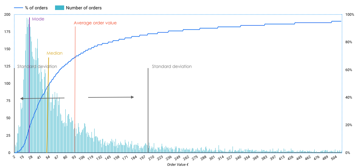
Visually, it’s also straightforward to see on our histogram.

Commonplace deviation
To finalize this text, we are going to add this final piece of knowledge to our histogram.
The usual deviation measures a dataset’s dispersion relative to its imply, in simpler phrases, it might assist us know what’s a normal order worth, or in different phrases, what does it imply when somebody says “it is a large order” or “it is a small order”.
In our case, an order is on common 93 euros.
In accordance with our question, the usual deviation is for us 112 euros. All orders that fall into the vary of 93 euros (our common) +112 (205 euros) and -112 (-19 euros) are thought of normal orders. In fact, on this case, we plotted the boundary at 0 as a substitute of -19.
In our case, orders above 205 euros might be thought of particular, or perhaps edge circumstances that we may look into. It’s also fascinating to look into them to grasp what they imply for our enterprise.
Additionally, orders from 0 to 205 euros characterize 85% of our orders. That means that is the vary the place we noticed and might count on our orders to be.
Conclusion
We do have a broader overview of how our clients are buying. It appears that evidently there are some orders (higher than 205 euros) that is perhaps outliers or perhaps relative to a particular side of the enterprise (perhaps giant firms’ orders, purchases for tech occasions, and many others…).
Half of our orders stay at low values (between 2–54 euros), it is perhaps fascinating to take a look at our portfolio and have a look at cross-selling/upselling methods if we need to enhance our order’s worth.
In accordance with the mode and in addition wanting on the histogram, most of our orders are from 20–24 euros, we perhaps have a top-selling merchandise or a mix of low-cost objects current in these orders.
Hopefully, this may also help you outline and resolve on methods to use on the orders stage, comparable to combining merchandise, altering transport charges, low cost affords (purchase 2 get 1 free), and much more inventive ones.
