In my final put up, I described user- and item-based collaborative filtering that are a few of the easiest advice algorithms. For somebody who’s used to traditional machine studying classification and regression algorithms, collaborative filtering might have felt a bit off. To me, machine studying nearly at all times offers with some operate which we try to maximise or decrease. In easy linear regression, we decrease the imply squared distance between our predictions and the true values. Logistic regression entails maximizing a chance operate. Nevertheless, in my put up on collaborative filtering, we randomly tried a bunch of various parameters (distance operate, top-k cutoff) and watched what occurred to the imply squared error. This positive doesn’t really feel like machine studying.
To convey some technical rigor to recommender programs, I want to discuss matrix factorization the place we do, actually, be taught parameters to a mannequin with a view to instantly decrease a operate. Explanations of matrix factorization typically begin with talks of “low-rank matrices” and “singular worth decomposition”. Whereas these are essential for a basic understanding of this matter, I don’t discover math-speak to be too useful in understanding the fundamental ideas of varied algorithms. Let me merely state the assumptions that primary matrix factorization makes.
Preliminary assumptions
We are going to use the identical instance information from the earlier put up, so recall that we had a user-by-item matrix the place nonzero components of the matrix are rankings {that a} consumer has given an merchandise. Matrix factorization assumes that:
- Every consumer may be described by okay attributes or options. For instance, characteristic 1 may be a quantity that claims how a lot every consumer likes sci-fi films.
- Every merchandise (film) may be described by an analagous set of okay attributes or options. To correspond to the above instance, characteristic 1 for the film may be a quantity that claims how shut the film is to pure sci-fi.
- If we multiply every characteristic of the consumer by the corresponding characteristic of the film and add every part collectively, this can be a very good approximation for the score the consumer would give that film.
That’s it. The sweetness is that we have no idea what these options are. Nor do we all know what number of (okay) options are related. We merely decide a quantity for okay and be taught the related values for all of the options for all of the customers and objects. How can we be taught? By minimizing a loss operate, after all!
We will flip our matrix factorization approximation of a okay-attribute consumer into math by letting a consumer u take the type of a okay-dimensional vector $textbf{x}_{u}$. Equally, an merchandise i may be represented by a okay-dimensional vector $textbf{y}_{i}$. Consumer u‘s predicted score for merchandise i is simply the dot product of their two vectors
$$hat r_{ui} = textbf{x}_{u}^{intercal} cdot{} textbf{y}_{i} = sumlimits_{okay} x_{uk}y_{ki}$$
the place $hat r_{ui}$ represents our prediction for the true score $r_{ui}$, and $textbf{y}_{i}$ ($textbf{x}_{u}^{intercal}$) is assumed to be a column (row) vector. These consumer and merchandise vectors are sometimes known as latent vectors or low-dimensional embeddings within the literature. The okay attributes are sometimes known as the latent elements. We are going to select to attenuate the sq. of the distinction between all rankings in our dataset ($S$) and our predictions. This produces a loss operate of the shape
$$L = sumlimits_{u,i in S}(r_{ui} – textbf{x}_{u}^{intercal} cdot{} textbf{y}_{i})^{2} + lambda_{x} sumlimits_{u} leftVert textbf{x}_{u} rightVert^{2} + lambda_{y} sumlimits_{i} leftVert textbf{y}_{i} rightVert^{2}$$
Be aware that we’ve added on two $L_{2}$ regularization phrases on the finish to stop overfitting of the consumer and merchandise vectors. Our objective now could be to attenuate this loss operate. Derivatives are an apparent instrument for minimizing capabilities, so I’ll cowl the 2 hottest derivative-based strategies. We’ll begin with Alternating Least Squares (ALS).
Alternating Least Squares
For ALS minimiztion, we maintain one set of latent vectors fixed. For this instance, we’ll decide the merchandise vectors. We then take the by-product of the loss operate with respect to the opposite set of vectors (the consumer vectors). We set the by-product equal to zero (we’re trying to find a minimal) and clear up for the non-constant vectors (the consumer vectors). Now comes the alternating half: With these new, solved-for consumer vectors in hand, we maintain them fixed, as an alternative, and take the by-product of the loss operate with respect to the beforehand fixed vectors (the merchandise vectors). We alternate forwards and backwards and perform this two-step dance till convergence.
Derivation
To clarify issues with math, let’s maintain the merchandise vectors ($textbf{y}_{i}$) fixed and take the by-product of the loss operate with respect to the consumer vectors ($textbf{x}_{u}$)
$$frac{partial L}{partial textbf{x}_{u}} = – 2 sumlimits_{i}(r_{ui} – textbf{x}_{u}^{intercal} cdot{} textbf{y}_{i}) textbf{y}_{i}^{intercal} + 2 lambda_{x} textbf{x}_{u}^{intercal}$$
$$0 = -(textbf{r}_{u} – textbf{x}_{u}^{intercal} Y^{intercal})Y + lambda_{x} textbf{x}_{u}^{intercal}$$
$$textbf{x}_{u}^{intercal}(Y^{intercal}Y + lambda_{x}I) = textbf{r}_{u}Y$$
$$textbf{x}_{u}^{intercal} = textbf{r}_{u}Y(Y^{intercal}Y + lambda_{x}I)^{-1}$$
A pair issues occur above: allow us to assume that we’ve $n$ customers and $m$ objects, so our rankings matrix is $n instances m$. We introduce the image $Y$ (with dimensioins $m instances okay$) to characterize all merchandise row vectors vertically stacked on one another. Additionally, the row vector $textbf{r}_{u}$ simply represents customers u‘s row from the rankings matrix with all of the rankings for all of the objects (so it has dimension $1 instances m$). Lastly, $I$ is simply the identification matrix which has dimension $okay instances okay$ right here.
Simply to ensure that every part works, let’s test our dimensions. I like doing this with Einstein notation. Though this looks like an esoteric physics factor, there was a purpose it was invented – it makes life actually easy! The fundamental tenant is that if one observes a variable for a matrix index greater than as soon as, then it’s implicitly assumed that you need to sum over that index. Together with the indices within the final assertion from the derivation above, this seems as the next for a single consumer’s dimension okay
$$x_{uk} = r_{ui}Y_{ik}(Y_{ki}Y_{ik} + lambda_{x}I_{kk})^{-1}$$
Once you perform all of the summations over all of the indices on the fitting hand aspect of the above assertion, all that’s left are u‘s because the rows and okay‘s because the columns. Good to go!
The derivation for the merchandise vectors is kind of related
$$frac{partial L}{partial textbf{y}_{i}} = – 2 sumlimits_{i}(r_{iu} – textbf{y}_{i}^{intercal} cdot{} textbf{x}_{u}) textbf{x}_{u}^{intercal} + 2 lambda_{y} textbf{y}_{i}^{intercal}$$
$$0 = -(textbf{r}_{i} – textbf{y}_{i}^{intercal} X^{intercal})X + lambda_{y} textbf{y}_{i}^{intercal}$$
$$ textbf{y}_{i}^{intercal} ( X^{intercal}X + lambda_{y}I) = textbf{r}_{i} X$$
$$ textbf{y}_{i}^{intercal} = textbf{r}_{i} X ( X^{intercal}X + lambda_{y}I) ^{-1}$$
Now that we’ve our equations, let’s program this factor up!
Computation
Identical to the final put up, we’ll use the MovieLens dataset. I’ll gloss over this half as a result of it’s been beforehand coated. Under, I import libraries, load the dataset into reminiscence, and cut up it into practice and check units. I’ll additionally create a helper operate with a view to simply calculate our imply squared error (which is the metric we’re making an attempt to optimize).
import numpy as np
import pandas as pd
np.random.seed(0)
# Load information from disk
names = ['user_id', 'item_id', 'rating', 'timestamp']
df = pd.read_csv('u.information', sep='t', names=names)
n_users = df.user_id.distinctive().form[0]
n_items = df.item_id.distinctive().form[0]

# Create r_{ui}, our rankings matrix
rankings = np.zeros((n_users, n_items))
for row in df.itertuples():
    rankings[row[1]-1, row[2]-1] = row[3]

# Cut up into coaching and check units.
# Take away 10 rankings for every consumer
# and assign them to the check set
def train_test_split(rankings):
    check = np.zeros(rankings.form)
    practice = rankings.copy()
    for consumer in xrange(rankings.form[0]):
        test_ratings = np.random.alternative(rankings[user, :].nonzero()[0],
                                        measurement=10,
                                        change=False)
        practice[user, test_ratings] = 0.
        check[user, test_ratings] = rankings[user, test_ratings]

    # Check and coaching are really disjoint
    assert(np.all((practice * check) == 0))
    return practice, check

practice, check = train_test_split(rankings)
from sklearn.metrics import mean_squared_error

def get_mse(pred, precise):
    # Ignore nonzero phrases.
    pred = pred[actual.nonzero()].flatten()
    precise = precise[actual.nonzero()].flatten()
    return mean_squared_error(pred, precise)
With the information loaded and massaged into good type, I’ve written a category beneath to carryout the ALS coaching. It needs to be famous that this class is closely impressed by Chris Johnson’s implicit-mf repo.
from numpy.linalg import clear up

class ExplicitMF():
    def __init__(self,
                 rankings,
                 n_factors=40,
                 item_reg=0.0,
                 user_reg=0.0,
                 verbose=False):
        """
        Practice a matrix factorization mannequin to foretell empty
        entries in a matrix. The terminology assumes a
        rankings matrix which is ~ consumer x merchandise

        Params
        ======
        rankings : (ndarray)
            Consumer x Merchandise matrix with corresponding rankings

        n_factors : (int)
            Variety of latent elements to make use of in matrix
            factorization mannequin

        item_reg : (float)
            Regularization time period for merchandise latent elements

        user_reg : (float)
            Regularization time period for consumer latent elements

        verbose : (bool)
            Whether or not or to not printout coaching progress
        """

        self.rankings = rankings
        self.n_users, self.n_items = rankings.form
        self.n_factors = n_factors
        self.item_reg = item_reg
        self.user_reg = user_reg
        self._v = verbose

    def als_step(self,
                 latent_vectors,
                 fixed_vecs,
                 rankings,
                 _lambda,
                 kind='consumer'):
        """
        One of many two ALS steps. Remedy for the latent vectors
        specified by kind.
        """
        if kind == 'consumer':
            # Precompute
            YTY = fixed_vecs.T.dot(fixed_vecs)
            lambdaI = np.eye(YTY.form[0]) * _lambda

            for u in xrange(latent_vectors.form[0]):
                latent_vectors[u, :] = clear up((YTY + lambdaI),
                                             rankings[u, :].dot(fixed_vecs))
        elif kind == 'merchandise':
            # Precompute
            XTX = fixed_vecs.T.dot(fixed_vecs)
            lambdaI = np.eye(XTX.form[0]) * _lambda

            for i in xrange(latent_vectors.form[0]):
                latent_vectors[i, :] = clear up((XTX + lambdaI),
                                             rankings[:, i].T.dot(fixed_vecs))
        return latent_vectors

    def practice(self, n_iter=10):
        """ Practice mannequin for n_iter iterations from scratch."""
        # initialize latent vectors
        self.user_vecs = np.random.random((self.n_users, self.n_factors))
        self.item_vecs = np.random.random((self.n_items, self.n_factors))

        self.partial_train(n_iter)

    def partial_train(self, n_iter):
        """
        Practice mannequin for n_iter iterations. Could be
        known as a number of instances for additional coaching.
        """
        ctr = 1
        whereas ctr <= n_iter:
            if ctr % 10 == 0 and self._v:
                print 'tpresent iteration: {}'.format(ctr)
            self.user_vecs = self.als_step(self.user_vecs,
                                           self.item_vecs,
                                           self.rankings,
                                           self.user_reg,
                                           kind='consumer')
            self.item_vecs = self.als_step(self.item_vecs,
                                           self.user_vecs,
                                           self.rankings,
                                           self.item_reg,
                                           kind='merchandise')
            ctr += 1

    def predict_all(self):
        """ Predict rankings for each consumer and merchandise. """
        predictions = np.zeros((self.user_vecs.form[0],
                                self.item_vecs.form[0]))
        for u in xrange(self.user_vecs.form[0]):
            for i in xrange(self.item_vecs.form[0]):
                predictions[u, i] = self.predict(u, i)

        return predictions
    def predict(self, u, i):
        """ Single consumer and merchandise prediction. """
        return self.user_vecs[u, :].dot(self.item_vecs[i, :].T)

    def calculate_learning_curve(self, iter_array, check):
        """
        Maintain observe of MSE as a operate of coaching iterations.

        Params
        ======
        iter_array : (record)
            Record of numbers of iterations to coach for every step of
            the training curve. e.g. [1, 5, 10, 20]
        check : (2D ndarray)
            Testing dataset (assumed to be consumer x merchandise).

        The operate creates two new class attributes:

        train_mse : (record)
            Coaching information MSE values for every worth of iter_array
        test_mse : (record)
            Check information MSE values for every worth of iter_array
        """
        iter_array.type()
        self.train_mse =[]
        self.test_mse = []
        iter_diff = 0
        for (i, n_iter) in enumerate(iter_array):
            if self._v:
                print 'Iteration: {}'.format(n_iter)
            if i == 0:
                self.practice(n_iter - iter_diff)
            else:
                self.partial_train(n_iter - iter_diff)

            predictions = self.predict_all()

            self.train_mse += [get_mse(predictions, self.ratings)]
            self.test_mse += [get_mse(predictions, test)]
            if self._v:
                print 'Practice mse: ' + str(self.train_mse[-1])
                print 'Check mse: ' + str(self.test_mse[-1])
            iter_diff = n_iter
Let’s strive an intial coaching with 40 latent elements and no regularization. We’ll calculate a studying curve monitoring the MSE as a operate of coaching iterations after which plot the end result.
MF_ALS = ExplicitMF(practice, n_factors=40,
                    user_reg=0.0, item_reg=0.0)
iter_array = [1, 2, 5, 10, 25, 50, 100]
MF_ALS.calculate_learning_curve(iter_array, check)
%matplotlib inline
import matplotlib.pyplot as plt
import seaborn as sns
sns.set()

def plot_learning_curve(iter_array, mannequin):
    plt.plot(iter_array, mannequin.train_mse,
             label='Coaching', linewidth=5)
    plt.plot(iter_array, mannequin.test_mse,
             label='Check', linewidth=5)


    plt.xticks(fontsize=16);
    plt.yticks(fontsize=16);
    plt.xlabel('iterations', fontsize=30);
    plt.ylabel('MSE', fontsize=30);
    plt.legend(loc='greatest', fontsize=20);
plot_learning_curve(iter_array, MF_ALS)
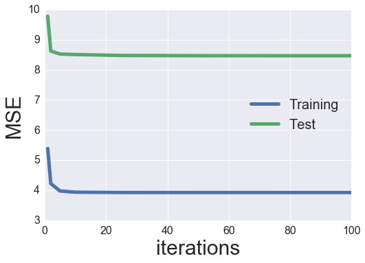
Analysis and Tuning
Seems to be like we’ve an inexpensive quantity of overfitting (our check MSE is ~ 50% better than our coaching MSE). Additionally, the check MSE bottoms out round 5 iterations then truly will increase after that (much more overfitting). We will strive including some regularization to see if this helps to alleviate a few of the overfitting.
MF_ALS = ExplicitMF(practice, n_factors=40,
                    user_reg=1., item_reg=1.)

iter_array = [1, 2, 5, 10, 25, 50, 100]
MF_ALS.calculate_learning_curve(iter_array, check)
plot_learning_curve(iter_array, MF_ALS)
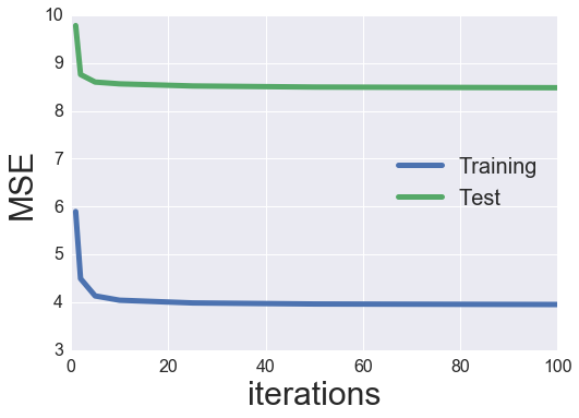
Hmmm, the regularization narrowed the hole between our coaching and check MSE, but it surely didn’t lower the check MSE an excessive amount of. We may spend all day trying to find optimum hyperparameters. We’ll simply setup a small grid search and tune each the regularization phrases and variety of latent elements. The merchandise and consumer regularization phrases can be restricted to be equal to one another.
latent_factors = [5, 10, 20, 40, 80]
regularizations = [0.01, 0.1, 1., 10., 100.]
regularizations.type()
iter_array = [1, 2, 5, 10, 25, 50, 100]

best_params = {}
best_params['n_factors'] = latent_factors[0]
best_params['reg'] = regularizations[0]
best_params['n_iter'] = 0
best_params['train_mse'] = np.inf
best_params['test_mse'] = np.inf
best_params['model'] = None

for truth in latent_factors:
    print 'Components: {}'.format(truth)
    for reg in regularizations:
        print 'Regularization: {}'.format(reg)
        MF_ALS = ExplicitMF(practice, n_factors=truth,
                            user_reg=reg, item_reg=reg)
        MF_ALS.calculate_learning_curve(iter_array, check)
        min_idx = np.argmin(MF_ALS.test_mse)
        if MF_ALS.test_mse[min_idx] < best_params['test_mse']:
            best_params['n_factors'] = truth
            best_params['reg'] = reg
            best_params['n_iter'] = iter_array[min_idx]
            best_params['train_mse'] = MF_ALS.train_mse[min_idx]
            best_params['test_mse'] = MF_ALS.test_mse[min_idx]
            best_params['model'] = MF_ALS
            print 'New optimum hyperparameters'
            print pd.Collection(best_params)
Components: 5
Regularization: 0.01
New optimum hyperparameters
mannequin        <__main__.ExplicitMF occasion at 0x7f3e0bd37fc8>
n_factors                                                   5
n_iter                                                      5
reg                                                      0.01
test_mse                                               8.8536
train_mse                                             6.13852
dtype: object
Regularization: 0.1
New optimum hyperparameters
mannequin        <__main__.ExplicitMF occasion at 0x7f3e0be0e248>
n_factors                                                   5
n_iter                                                     10
reg                                                       0.1
test_mse                                              8.82131
train_mse                                             6.13235
dtype: object
Regularization: 1.0
New optimum hyperparameters
mannequin        <__main__.ExplicitMF occasion at 0x7f3e1267e128>
n_factors                                                   5
n_iter                                                     10
reg                                                         1
test_mse                                              8.74613
train_mse                                             6.19465
dtype: object
Regularization: 10.0
Regularization: 100.0
Components: 10
Regularization: 0.01
New optimum hyperparameters
mannequin        <__main__.ExplicitMF occasion at 0x7f3e0be30fc8>
n_factors                                                  10
n_iter                                                    100
reg                                                      0.01
test_mse                                              8.20374
train_mse                                             5.39429
dtype: object
Regularization: 0.1
Regularization: 1.0
Regularization: 10.0
Regularization: 100.0
Components: 20
Regularization: 0.01
New optimum hyperparameters
mannequin        <__main__.ExplicitMF occasion at 0x7f3e0bdabfc8>
n_factors                                                  20
n_iter                                                     50
reg                                                      0.01
test_mse                                              8.07322
train_mse                                             4.75437
dtype: object
Regularization: 0.1
Regularization: 1.0
Regularization: 10.0
Regularization: 100.0
Components: 40
Regularization: 0.01
Regularization: 0.1
Regularization: 1.0
Regularization: 10.0
Regularization: 100.0
Components: 80
Regularization: 0.01
Regularization: 0.1
Regularization: 1.0
Regularization: 10.0
Regularization: 100.0
best_als_model = best_params['model']
plot_learning_curve(iter_array, best_als_model)
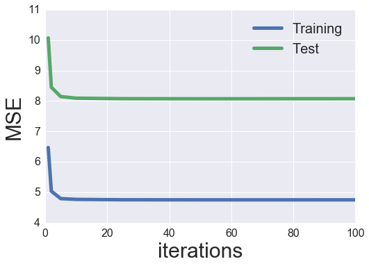
So it appears to be like like the perfect performing parameters had been 20 elements and a regularization worth of 0.01. I want to once more take a look at the movie-to-movie similarity like my earlier put up, however let’s first discover the opposite minimization algorithm: stochastic gradient descent (SGD).
Stochastic Gradient Descent
With SGD, we once more take derivatives of the loss operate, however we take the by-product with respect to every variable within the mannequin. The “stochastic” side of the algorithm entails taking the by-product and updating characteristic weights one particular person pattern at a time. So, for every pattern, we take the by-product of every variable, set all of them equal to zero, clear up for the characteristic weights, and replace every characteristic. By some means this methodology truly converges.
We are going to use an identical loss operate to earlier than, however I’m going so as to add some extra particulars to the mannequin. As a substitute of assuming {that a} consumer u‘s score for merchandise i may be described just by the dot product of the consumer and merchandise latent vectors, we are going to take into account that every consumer and merchandise can have a bias time period related to them. The rational is that certan customers would possibly are likely to charge all films extremely, or sure films might are likely to at all times have low rankings. The way in which that I give it some thought is that the bias time period takes care of the “DC” a part of the sign which permits the latent elements to account for the extra detailed variance in sign (form of just like the AC half). We can even embrace a worldwide bias time period as properly. With all issues mixed, our predicted score turns into
$$ hat r_{ui} = mu + b_{u} + b_{i} + textbf{x}_{u}^{intercal} cdot{} textbf{y}_{i} $$
the place $mu$ is the worldwide bias, and $b_{u}$ ($b_{i}$) is the consumer (merchandise) bias. Our loss operate now turns into
$$L = sumlimits_{u,i}(r_{ui} – (mu + b_{u} + b_{i} + textbf{x}_{u}^{intercal} cdot{} textbf{y}_{i}))^{2} newline
- lambda_{xb} sumlimits_{u} leftVert b_{u} rightVert^{2} + lambda_{yb} sumlimits_{i} leftVert b_{i} rightVert^{2} newline
- lambda_{xf} sumlimits_{u} leftVert textbf{x}_{u} rightVert^{2} + lambda_{yf} sumlimits_{i} leftVert textbf{y}_{i} rightVert^{2}$$
the place we’ve added on additional bias regularization phrases. We wish to replace every characteristic (consumer and merchandise latent elements and bias phrases) with every pattern. The replace for the consumer bias is given by
$$ b_{u} leftarrow b_{u} – eta frac{partial L}{partial b_{u}} $$
the place $eta$ is the studying charge which weights how a lot our replace modifies the characteristic weights. The by-product time period is given by
$$ frac{partial L}{partial b_{u}} = 2(r_{ui} – (mu + b_{u} + b_{i} + textbf{x}_{u}^{intercal} cdot{} textbf{y}_{i}))(-1) + 2lambda_{xb} b_{u} $$
$$ frac{partial L}{partial b_{u}} = 2(e_{ui})(-1) + 2lambda_{xb} b_{u} $$
$$ frac{partial L}{partial b_{u}} = – e_{ui} + lambda_{xb} b_{u} $$
the place $e_{ui}$ represents the error in our prediction, and we’ve dropped the issue of two (we will assume it will get rolled up within the studying charge). For all of our options, the updates find yourself being
$$ b_{u} leftarrow b_{u} + eta , (e_{ui} – lambda_{xb} b_{u}) $$
$$ b_{i} leftarrow b_{i} + eta , (e_{ui} – lambda_{yb} b_{i}) $$
$$ textbf{x}_{u} leftarrow textbf{x}_{u} + eta , (e_{ui}textbf{y}_{i} – lambda_{xf} textbf{x}_{u}) $$
$$ textbf{y}_{i} leftarrow textbf{y}_{i} + eta , (e_{ui}textbf{x}_{u} – lambda_{yf} textbf{y}_{i}) $$
Computation
I’ve modified the unique ExplicitMF class to permit for both sgd or als studying.
class ExplicitMF():
    def __init__(self,
                 rankings,
                 n_factors=40,
                 studying='sgd',
                 item_fact_reg=0.0,
                 user_fact_reg=0.0,
                 item_bias_reg=0.0,
                 user_bias_reg=0.0,
                 verbose=False):
        """
        Practice a matrix factorization mannequin to foretell empty
        entries in a matrix. The terminology assumes a
        rankings matrix which is ~ consumer x merchandise

        Params
        ======
        rankings : (ndarray)
            Consumer x Merchandise matrix with corresponding rankings

        n_factors : (int)
            Variety of latent elements to make use of in matrix
            factorization mannequin
        studying : (str)
            Methodology of optimization. Choices embrace
            'sgd' or 'als'.

        item_fact_reg : (float)
            Regularization time period for merchandise latent elements

        user_fact_reg : (float)
            Regularization time period for consumer latent elements

        item_bias_reg : (float)
            Regularization time period for merchandise biases

        user_bias_reg : (float)
            Regularization time period for consumer biases

        verbose : (bool)
            Whether or not or to not printout coaching progress
        """

        self.rankings = rankings
        self.n_users, self.n_items = rankings.form
        self.n_factors = n_factors
        self.item_fact_reg = item_fact_reg
        self.user_fact_reg = user_fact_reg
        self.item_bias_reg = item_bias_reg
        self.user_bias_reg = user_bias_reg
        self.studying = studying
        if self.studying == 'sgd':
            self.sample_row, self.sample_col = self.rankings.nonzero()
            self.n_samples = len(self.sample_row)
        self._v = verbose

    def als_step(self,
                 latent_vectors,
                 fixed_vecs,
                 rankings,
                 _lambda,
                 kind='consumer'):
        """
        One of many two ALS steps. Remedy for the latent vectors
        specified by kind.
        """
        if kind == 'consumer':
            # Precompute
            YTY = fixed_vecs.T.dot(fixed_vecs)
            lambdaI = np.eye(YTY.form[0]) * _lambda

            for u in xrange(latent_vectors.form[0]):
                latent_vectors[u, :] = clear up((YTY + lambdaI),
                                             rankings[u, :].dot(fixed_vecs))
        elif kind == 'merchandise':
            # Precompute
            XTX = fixed_vecs.T.dot(fixed_vecs)
            lambdaI = np.eye(XTX.form[0]) * _lambda

            for i in xrange(latent_vectors.form[0]):
                latent_vectors[i, :] = clear up((XTX + lambdaI),
                                             rankings[:, i].T.dot(fixed_vecs))
        return latent_vectors

    def practice(self, n_iter=10, learning_rate=0.1):
        """ Practice mannequin for n_iter iterations from scratch."""
        # initialize latent vectors
        self.user_vecs = np.random.regular(scale=1./self.n_factors,
                                          measurement=(self.n_users, self.n_factors))
        self.item_vecs = np.random.regular(scale=1./self.n_factors,
                                          measurement=(self.n_items, self.n_factors))

        if self.studying == 'als':
            self.partial_train(n_iter)
        elif self.studying == 'sgd':
            self.learning_rate = learning_rate
            self.user_bias = np.zeros(self.n_users)
            self.item_bias = np.zeros(self.n_items)
            self.global_bias = np.imply(self.rankings[np.where(self.ratings != 0)])
            self.partial_train(n_iter)


    def partial_train(self, n_iter):
        """
        Practice mannequin for n_iter iterations. Could be
        known as a number of instances for additional coaching.
        """
        ctr = 1
        whereas ctr <= n_iter:
            if ctr % 10 == 0 and self._v:
                print 'tpresent iteration: {}'.format(ctr)
            if self.studying == 'als':
                self.user_vecs = self.als_step(self.user_vecs,
                                               self.item_vecs,
                                               self.rankings,
                                               self.user_fact_reg,
                                               kind='consumer')
                self.item_vecs = self.als_step(self.item_vecs,
                                               self.user_vecs,
                                               self.rankings,
                                               self.item_fact_reg,
                                               kind='merchandise')
            elif self.studying == 'sgd':
                self.training_indices = np.arange(self.n_samples)
                np.random.shuffle(self.training_indices)
                self.sgd()
            ctr += 1

    def sgd(self):
        for idx in self.training_indices:
            u = self.sample_row[idx]
            i = self.sample_col[idx]
            prediction = self.predict(u, i)
            e = (self.rankings[u,i] - prediction) # error

            # Replace biases
            self.user_bias[u] += self.learning_rate *
                                (e - self.user_bias_reg * self.user_bias[u])
            self.item_bias[i] += self.learning_rate *
                                (e - self.item_bias_reg * self.item_bias[i])

            #Replace latent elements
            self.user_vecs[u, :] += self.learning_rate *
                                    (e * self.item_vecs[i, :] -
                                     self.user_fact_reg * self.user_vecs[u,:])
            self.item_vecs[i, :] += self.learning_rate *
                                    (e * self.user_vecs[u, :] -
                                     self.item_fact_reg * self.item_vecs[i,:])
    def predict(self, u, i):
        """ Single consumer and merchandise prediction."""
        if self.studying == 'als':
            return self.user_vecs[u, :].dot(self.item_vecs[i, :].T)
        elif self.studying == 'sgd':
            prediction = self.global_bias + self.user_bias[u] + self.item_bias[i]
            prediction += self.user_vecs[u, :].dot(self.item_vecs[i, :].T)
            return prediction

    def predict_all(self):
        """ Predict rankings for each consumer and merchandise."""
        predictions = np.zeros((self.user_vecs.form[0],
                                self.item_vecs.form[0]))
        for u in xrange(self.user_vecs.form[0]):
            for i in xrange(self.item_vecs.form[0]):
                predictions[u, i] = self.predict(u, i)

        return predictions

    def calculate_learning_curve(self, iter_array, check, learning_rate=0.1):
        """
        Maintain observe of MSE as a operate of coaching iterations.

        Params
        ======
        iter_array : (record)
            Record of numbers of iterations to coach for every step of
            the training curve. e.g. [1, 5, 10, 20]
        check : (2D ndarray)
            Testing dataset (assumed to be consumer x merchandise).

        The operate creates two new class attributes:

        train_mse : (record)
            Coaching information MSE values for every worth of iter_array
        test_mse : (record)
            Check information MSE values for every worth of iter_array
        """
        iter_array.type()
        self.train_mse =[]
        self.test_mse = []
        iter_diff = 0
        for (i, n_iter) in enumerate(iter_array):
            if self._v:
                print 'Iteration: {}'.format(n_iter)
            if i == 0:
                self.practice(n_iter - iter_diff, learning_rate)
            else:
                self.partial_train(n_iter - iter_diff)

            predictions = self.predict_all()

            self.train_mse += [get_mse(predictions, self.ratings)]
            self.test_mse += [get_mse(predictions, test)]
            if self._v:
                print 'Practice mse: ' + str(self.train_mse[-1])
                print 'Check mse: ' + str(self.test_mse[-1])
            iter_diff = n_iter
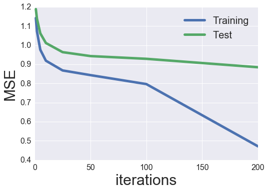
Just like the ALS part above, let’s strive trying on the studying curve for 40 latent elements, no regularizaton, and a studying charge of 0.001.
MF_SGD = ExplicitMF(practice, 40, studying='sgd', verbose=True)
iter_array = [1, 2, 5, 10, 25, 50, 100, 200]
MF_SGD.calculate_learning_curve(iter_array, check, learning_rate=0.001)
Iteration: 1
Practice mse: 1.14177869865
Check mse: 1.18835604452
Iteration: 2
Practice mse: 1.07185141375
Check mse: 1.1384050219
Iteration: 5
Practice mse: 0.975472334851
Check mse: 1.06177445752
Iteration: 10
Practice mse: 0.917930429855
Check mse: 1.01129117946
Iteration: 25
    present iteration: 10
Practice mse: 0.866100381526
Check mse: 0.963769980492
Iteration: 50
    present iteration: 10
    present iteration: 20
Practice mse: 0.838103967224
Check mse: 0.943193798801
Iteration: 100
    present iteration: 10
    present iteration: 20
    present iteration: 30
    present iteration: 40
    present iteration: 50
Practice mse: 0.747444200503
Check mse: 0.924721070559
Iteration: 200
    present iteration: 10
    present iteration: 20
    present iteration: 30
    present iteration: 40
    present iteration: 50
    present iteration: 60
    present iteration: 70
    present iteration: 80
    present iteration: 90
    present iteration: 100
Practice mse: 0.401711968464
Check mse: 0.922782112511
plot_learning_curve(iter_array, MF_SGD)
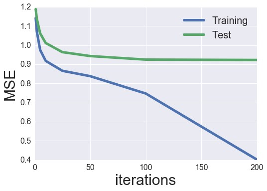
Wow, fairly a bit higher than earlier than! I assume that that is doubtless as a result of inclusion of bias phrases (particularly as a result of the rankings will not be normalized).
Analysis and tuning
Let’s attempt to optimize some hyperparameters. We’ll begin with a grid search of the training charge.
iter_array = [1, 2, 5, 10, 25, 50, 100, 200]
learning_rates = [1e-5, 1e-4, 1e-3, 1e-2]

best_params = {}
best_params['learning_rate'] = None
best_params['n_iter'] = 0
best_params['train_mse'] = np.inf
best_params['test_mse'] = np.inf
best_params['model'] = None


for charge in learning_rates:
    print 'Fee: {}'.format(charge)
    MF_SGD = ExplicitMF(practice, n_factors=40, studying='sgd')
    MF_SGD.calculate_learning_curve(iter_array, check, learning_rate=charge)
    min_idx = np.argmin(MF_SGD.test_mse)
    if MF_SGD.test_mse[min_idx] < best_params['test_mse']:
        best_params['n_iter'] = iter_array[min_idx]
        best_params['learning_rate'] = charge
        best_params['train_mse'] = MF_SGD.train_mse[min_idx]
        best_params['test_mse'] = MF_SGD.test_mse[min_idx]
        best_params['model'] = MF_SGD
        print 'New optimum hyperparameters'
        print pd.Collection(best_params)
Fee: 1e-05
New optimum hyperparameters
learning_rate                                               1e-05
mannequin            <__main__.ExplicitMF occasion at 0x7f3e0bc192d8>
n_iter                                                        200
test_mse                                                  1.13841
train_mse                                                 1.07205
dtype: object
Fee: 0.0001
New optimum hyperparameters
learning_rate                                              0.0001
mannequin            <__main__.ExplicitMF occasion at 0x7f3e0be9f3f8>
n_iter                                                        200
test_mse                                                 0.972998
train_mse                                                0.876805
dtype: object
Fee: 0.001
New optimum hyperparameters
learning_rate                                               0.001
mannequin            <__main__.ExplicitMF occasion at 0x7f3e0bcf7bd8>
n_iter                                                        200
test_mse                                                 0.914752
train_mse                                                0.403944
dtype: object
Fee: 0.01
Seems to be like a studying charge 0.001 was the perfect worth. We’ll now full the hyperparameter optimization with a grid search by means of regularization phrases and latent elements. This takes some time and will simply be parallelized, however that’s past the scope of this put up. Perhaps subsequent put up I’ll look into optimizing a few of these algorithms.
iter_array = [1, 2, 5, 10, 25, 50, 100, 200]
latent_factors = [5, 10, 20, 40, 80]
regularizations = [0.001, 0.01, 0.1, 1.]
regularizations.type()

best_params = {}
best_params['n_factors'] = latent_factors[0]
best_params['reg'] = regularizations[0]
best_params['n_iter'] = 0
best_params['train_mse'] = np.inf
best_params['test_mse'] = np.inf
best_params['model'] = None

for truth in latent_factors:
    print 'Components: {}'.format(truth)
    for reg in regularizations:
        print 'Regularization: {}'.format(reg)
        MF_SGD = ExplicitMF(practice, n_factors=truth, studying='sgd',
                            user_fact_reg=reg, item_fact_reg=reg,
                            user_bias_reg=reg, item_bias_reg=reg)
        MF_SGD.calculate_learning_curve(iter_array, check, learning_rate=0.001)
        min_idx = np.argmin(MF_SGD.test_mse)
        if MF_SGD.test_mse[min_idx] < best_params['test_mse']:
            best_params['n_factors'] = truth
            best_params['reg'] = reg
            best_params['n_iter'] = iter_array[min_idx]
            best_params['train_mse'] = MF_SGD.train_mse[min_idx]
            best_params['test_mse'] = MF_SGD.test_mse[min_idx]
            best_params['model'] = MF_SGD
            print 'New optimum hyperparameters'
            print pd.Collection(best_params)
Components: 5
Regularization: 0.001
New optimum hyperparameters
mannequin        <__main__.ExplicitMF occasion at 0x7f3e0bd15758>
n_factors                                                   5
n_iter                                                    100
reg                                                     0.001
test_mse                                             0.935368
train_mse                                            0.750861
dtype: object
Regularization: 0.01
New optimum hyperparameters
mannequin        <__main__.ExplicitMF occasion at 0x7f3e0bd682d8>
n_factors                                                   5
n_iter                                                    200
reg                                                      0.01
test_mse                                             0.933326
train_mse                                             0.67293
dtype: object
Regularization: 0.1
New optimum hyperparameters
mannequin        <__main__.ExplicitMF occasion at 0x7f3e0bd68dd0>
n_factors                                                   5
n_iter                                                    200
reg                                                       0.1
test_mse                                             0.914926
train_mse                                            0.769424
dtype: object
Regularization: 1.0
Components: 10
Regularization: 0.001
Regularization: 0.01
Regularization: 0.1
New optimum hyperparameters
mannequin        <__main__.ExplicitMF occasion at 0x7f3e0bb72f38>
n_factors                                                  10
n_iter                                                    200
reg                                                       0.1
test_mse                                             0.910528
train_mse                                            0.765306
dtype: object
Regularization: 1.0
Components: 20
Regularization: 0.001
Regularization: 0.01
Regularization: 0.1
Regularization: 1.0
Components: 40
Regularization: 0.001
Regularization: 0.01
New optimum hyperparameters
mannequin        <__main__.ExplicitMF occasion at 0x7f3e0bb72f80>
n_factors                                                  40
n_iter                                                    200
reg                                                      0.01
test_mse                                              0.89187
train_mse                                            0.459506
dtype: object
Regularization: 0.1
Regularization: 1.0
Components: 80
Regularization: 0.001
New optimum hyperparameters
mannequin        <__main__.ExplicitMF occasion at 0x7f3e0bb72680>
n_factors                                                  80
n_iter                                                    200
reg                                                     0.001
test_mse                                             0.891822
train_mse                                            0.408462
dtype: object
Regularization: 0.01
New optimum hyperparameters
mannequin        <__main__.ExplicitMF occasion at 0x7f3e0bb72f38>
n_factors                                                  80
n_iter                                                    200
reg                                                      0.01
test_mse                                             0.884726
train_mse                                            0.471539
dtype: object
Regularization: 0.1
Regularization: 1.0
plot_learning_curve(iter_array, best_params['model'])
print 'Finest regularization: {}'.format(best_params['reg'])
print 'Finest latent elements: {}'.format(best_params['n_factors'])
print 'Finest iterations: {}'.format(best_params['n_iter'])
Finest regularization: 0.01
Finest latent elements: 80
Finest iterations: 200
It needs to be famous that each our greatest latent elements and greatest iteration depend had been on the maximums of their respective grid searches. In hindsight, we should always have set the grid search to a wider vary. In apply, I’m going to simply go together with these parameters. We may spend all day optimizing, however that is only a weblog put up on extensively studied information.
Eye exams
To wrap up this put up, let’s once more take a look at movie-to-movie similarity utilizing by utilizing themoviedb.org‘s API to seize the film posters and visualize the highest 5 most related films to an enter film. We’ll use the cosine similarity of the merchandise latent vectors to calculate the similarity. Let’s go for gold and use your entire dataset to coach the latent vectors and calculate similarity. We’ll do that for each ALS and SGD fashions and evaluate the outcomes.
We begin by coaching each fashions with the perfect parameters we discovered.
best_als_model = ExplicitMF(rankings, n_factors=20, studying='als',
                            item_fact_reg=0.01, user_fact_reg=0.01)
best_als_model.practice(50)
best_sgd_model = ExplicitMF(rankings, n_factors=80, studying='sgd',
                            item_fact_reg=0.01, user_fact_reg=0.01,
                            user_bias_reg=0.01, item_bias_reg=0.01)
best_sgd_model.practice(200, learning_rate=0.001)
I’ll use this small operate to calculate each the ALS and the SGD movie-to-movie similarity matrices.
def cosine_similarity(mannequin):
    sim = mannequin.item_vecs.dot(mannequin.item_vecs.T)
    norms = np.array([np.sqrt(np.diagonal(sim))])
    return sim / norms / norms.T

als_sim = cosine_similarity(best_als_model)
sgd_sim = cosine_similarity(best_sgd_model)
Lastly, identical to earlier than, let’s learn within the film’s IMDB urls and use these to question the themoviedb.org API.
# Load in film information
idx_to_movie = {}
with open('u.merchandise', 'r') as f:
    for line in f.readlines():
        information = line.cut up('|')
        idx_to_movie[int(info[0])-1] = information[4]
# Construct operate to question themoviedb.org's API
import requests
import json

# Get base url filepath construction. w185 corresponds to measurement of film poster.
api_key = 'INSERT API KEY HERE'
headers = {'Settle for': 'software/json'}
payload = {'api_key': api_key}
response = requests.get("http://api.themoviedb.org/3/configuration",
                        params=payload,
                        headers=headers)
response = json.hundreds(response.textual content)
base_url = response['images']['base_url'] + 'w185'

def get_poster(imdb_url, base_url, api_key):
    # Get IMDB film ID
    response = requests.get(imdb_url)
    movie_id = response.url.cut up('/')[-2]

    # Question themoviedb.org API for film poster path.
    movie_url = 'http://api.themoviedb.org/3/film/{:}/pictures'.format(movie_id)
    headers = {'Settle for': 'software/json'}
    payload = {'api_key': api_key}
    response = requests.get(movie_url, params=payload, headers=headers)
    strive:
        file_path = json.hundreds(response.textual content)['posters'][0]['file_path']
    besides:
        # IMDB film ID is usually no good. Have to get appropriate one.
        movie_title = imdb_url.cut up('?')[-1].cut up('(')[0]
        payload['query'] = movie_title
        response = requests.get('http://api.themoviedb.org/3/search/film',
                                params=payload,
                                headers=headers)
        strive:
            movie_id = json.hundreds(response.textual content)['results'][0]['id']
            payload.pop('question', None)
            movie_url = 'http://api.themoviedb.org/3/film/{:}/pictures'
                        .format(movie_id)
            response = requests.get(movie_url, params=payload, headers=headers)
            file_path = json.hundreds(response.textual content)['posters'][0]['file_path']
        besides:
            # Typically the url simply would not work.
            # Return '' in order that it doesn't mess up Picture()
            return ''

    return base_url + file_path
To visualise the posters within the Jupyter pocket book’s cells, we will use the IPython.show methodology. I’ve modified issues barely from final time in order that the film posters seem horizontally. Particular because of this Stack Overflow reply for the concept to make use of straight HTML.
from IPython.show import HTML
from IPython.show import show

def display_top_k_movies(similarity, mapper, movie_idx, base_url, api_key, okay=5):
    movie_indices = np.argsort(similarity[movie_idx,:])[::-1]
    pictures = ''
    k_ctr = 0
    # Begin i at 1 to not seize the enter film
    i = 1
    whereas k_ctr < 5:
        film = mapper[movie_indices[i]]
        poster = get_poster(film, base_url, api_key)
        if poster != '':
            pictures += "<img fashion='width: 120px; margin: 0px;
                      float: left; border: 1px stable black;' src='%s' />"
                      % poster
            k_ctr += 1
        i += 1
    show(HTML(pictures))

def compare_recs(als_similarity, sgd_similarity, mapper,
                 movie_idx, base_url, api_key, okay=5):
    # Show enter
    show(HTML('<font measurement=5>'+'Enter'+'</font>'))
    input_poster = get_poster(mapper[movie_idx], base_url, api_key)
    input_image = "<img fashion='width: 120px; margin: 0px;
                      float: left; border: 1px stable black;' src='%s' />"
                  % input_poster
    show(HTML(input_image))
    # Show ALS Recs
    show(HTML('<font measurement=5>'+'ALS Recs'+'</font>'))
    display_top_k_movies(als_similarity, idx_to_movie,
                         movie_idx, base_url, api_key)
    # Show SGD Recs
    show(HTML('<font measurement=5>'+'SGD Recs'+'</font>'))
    display_top_k_movies(sgd_similarity, idx_to_movie,
                         movie_idx, base_url, api_key)
I’ll allow you to look by means of 5 totally different movie-to-movie suggestions beneath.
So how do we expect we did? I discover it very fascinating that the perfect check MSE for our ALS mannequin was 8.07 in comparison with 0.88 for SGD. That’s a large distinction, and but I believe the ALS suggestions would possibly truly beat out the SGD ones; notably, the GoldenEye and Dumbo suggestions.
I’ve discovered related conduct in a few of my very own work, as properly. I’ve a imprecise hunch that SGD tends to overfit greater than ALS and is extra inclined to recognition bias. Sadly, I’ve zero math to again this up, so it’ll stay purely anecdotal for now. Another clarification may very well be that the SGD movie-to-movie suggestions are literally higher than the ALS ones even when they appear like much less related films. In a latest Netflix paper, they present an identical comparability of two totally different fashions’ movie-to-movie suggestions. It seems that the mannequin with films that look much less related by eye (however are typically extra widespread films) performs higher on A/B exams. And actually, A/B exams are a significantly better approach of really benchmarking advice programs in comparison with this offline information modeling.
And on a ultimate observe, possibly we might wish to simply mix each fashions into an ensemble which appears to be what everbody does these days.
Hyperlink to Jupyter pocket book of this put up.
