The way to practice them and the way they work, with working code examples

On this publish we’re going to debate a generally used machine studying mannequin known as determination tree. Determination timber are most well-liked for a lot of purposes, primarily because of their excessive explainability, but additionally because of the truth that they’re comparatively easy to arrange and practice, and the brief time it takes to carry out a prediction with a choice tree. Determination timber are pure to tabular information, and, in truth, they at the moment appear to outperform neural networks on that kind of knowledge (versus photos). In contrast to neural networks, timber don’t require enter normalization, since their coaching is just not based mostly on gradient descent and so they have only a few parameters to optimize on. They will even practice on information with lacking values, however these days this apply is much less really useful, and lacking values are often imputed.
Among the many well-known use-cases for determination timber are advice techniques (what are your predicted film preferences based mostly in your previous selections and different options, e.g. age, gender and so forth.) and search engines like google.
The prediction course of in a tree consists of a sequence of comparisons of the pattern’s attributes (options) with pre-learned threshold values. Ranging from the highest (the foundation of the tree) and going downward (towards the leaves, sure, reverse to real-life timber), in every step the results of the comparability determines if the pattern goes left or proper within the tree, and by that — determines the subsequent comparability step. When our pattern reaches a leaf (an finish node) — the choice, or prediction, is made, based mostly on the bulk class within the leaf.
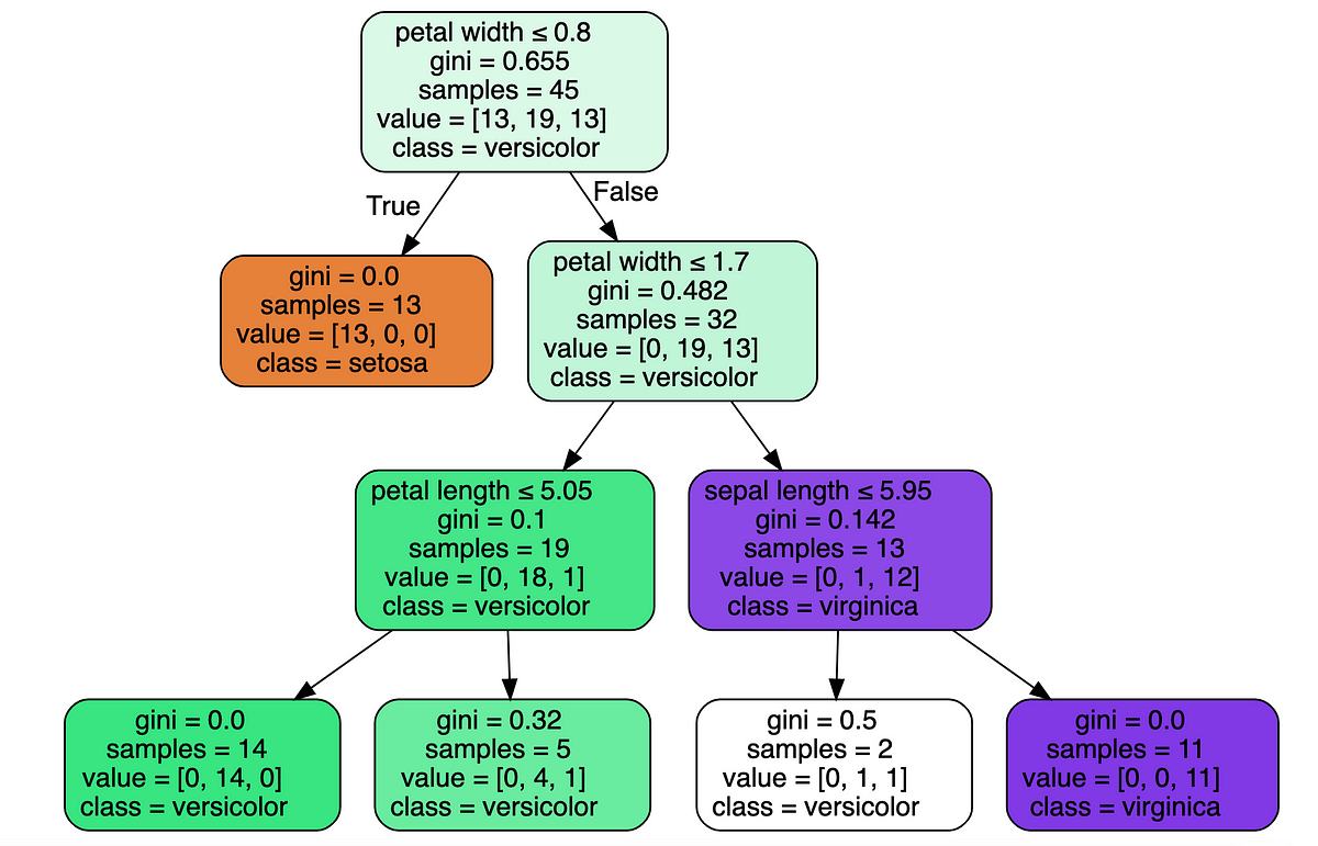
Fig.1 reveals this course of with an issue of classifying Iris samples into 3 completely different species (lessons) based mostly on their petal and sepal lengths and widths.
Our instance will probably be based mostly on the well-known Iris dataset (Fisher, R.A. “The usage of a number of measurements in taxonomic issues” Annual Eugenics, 7, Half II, 179–188 (1936)). I downloaded it utilizing sklearn package deal, which is a BSD (Berkley Supply Distribution) license software program. I modified the options of one of many lessons and decreased the practice set dimension, to combine the lessons somewhat bit and make it extra attention-grabbing.

We’ll work out the small print of this tree later. For now, we’ll study the foundation node and spot that our coaching inhabitants has 45 samples, divided into 3 lessons like so: [13, 19, 13]. The ‘class’ attribute tells us the label the tree would predict for this pattern if it have been a leaf — based mostly on the bulk class within the node. For instance — if we weren’t allowed to run any comparisons, we’d be within the root node and our greatest prediction could be class Veriscolor, because it has 19 samples within the practice set, vs. 13 for the opposite two lessons. If our sequence of comparisons led us to the leaf second from left, the mannequin’s prediction would, once more, be Veriscolor, since within the coaching set there have been 4 samples of that class that reached this leaf, vs. just one pattern of sophistication Virginica and 0 samples of sophistication Setosa.
Determination timber can be utilized for both classification or regression issues. Let’s begin by discussing the classification drawback and clarify how the tree coaching algorithm works.
Let’s see how we practice a tree utilizing sklearn after which focus on the mechanism.
Downloading the dataset:
import numpy as np
from sklearn.datasets import load_iris
from sklearn.model_selection import train_test_split
from sklearn.preprocessing import OneHotEncoderiris = load_iris()
X = iris['data']
y = iris['target']
names = iris['target_names']
feature_names = iris['feature_names']# One sizzling encoding
enc = OneHotEncoder()
Y = enc.fit_transform(y[:, np.newaxis]).toarray()# Modifying the dataset
X[y==1,2] = X[y==1,2] + 0.3# Cut up the information set into coaching and testing
X_train, X_test, Y_train, Y_test = train_test_split(
X, Y, test_size=0.5, random_state=2)# Lowering the practice set to make issues extra attention-grabbing
X_train = X_train[30:,:]
Y_train = Y_train[30:,:]
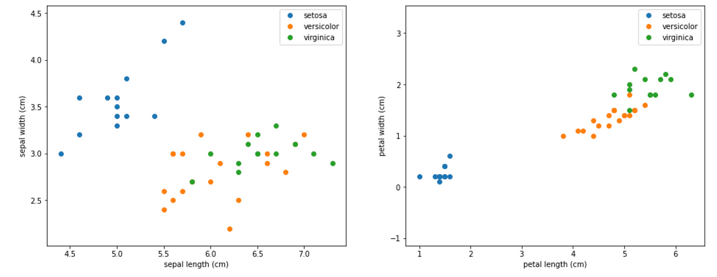
Let’s visualize the dataset.
# Visualize the information units
import matplotlib
import matplotlib.pyplot as pltplt.determine(figsize=(16, 6))
plt.subplot(1, 2, 1)
for goal, target_name in enumerate(names):
X_plot = X[y == target]
plt.plot(X_plot[:, 0], X_plot[:, 1], linestyle='none', marker='o', label=target_name)
plt.xlabel(feature_names[0])
plt.ylabel(feature_names[1])
plt.axis('equal')
plt.legend();plt.subplot(1, 2, 2)
for goal, target_name in enumerate(names):
X_plot = X[y == target]
plt.plot(X_plot[:, 2], X_plot[:, 3], linestyle='none', marker='o', label=target_name)
plt.xlabel(feature_names[2])
plt.ylabel(feature_names[3])
plt.axis('equal')
plt.legend();

and simply the practice set:
plt.determine(figsize=(16, 6))
plt.subplot(1, 2, 1)
for goal, target_name in enumerate(names):
X_plot = X_train[Y_train[:,target] == 1]
plt.plot(X_plot[:, 0], X_plot[:, 1], linestyle='none', marker='o', label=target_name)
plt.xlabel(feature_names[0])
plt.ylabel(feature_names[1])
plt.axis('equal')
plt.legend();plt.subplot(1, 2, 2)
for goal, target_name in enumerate(names):
X_plot = X_train[Y_train[:,target] == 1]
plt.plot(X_plot[:, 2], X_plot[:, 3], linestyle='none', marker='o', label=target_name)
plt.xlabel(feature_names[2])
plt.ylabel(feature_names[3])
plt.axis('equal')
plt.legend();
Now we’re prepared to coach a tree and visualize it. The result’s the mannequin that we noticed in Fig.1.
from sklearn import tree
import graphviziristree = tree.DecisionTreeClassifier(max_depth=3, criterion='gini', random_state=0)
iristree.match(X_train, enc.inverse_transform(Y_train))feature_names = ['sepal length', 'sepal width', 'petal length', 'petal width']dot_data = tree.export_graphviz(iristree, out_file=None,
feature_names=feature_names,
class_names=names,
stuffed=True, rounded=True,
special_characters=True)
graph = graphviz.Supply(dot_data)show(graph)
We are able to see that the tree makes use of the petal width for its first and second splits — the primary cut up cleanly separates class Setosa from the opposite two. Notice that for the primary cut up, the petal size might work equally effectively.
Let’s see the classification precision of this mannequin on the practice set, adopted by the take a look at set:
from sklearn.metrics import precision_score
from sklearn.metrics import recall_scoreiristrainpred = iristree.predict(X_train)
iristestpred = iristree.predict(X_test)# practice precision:
show(precision_score(enc.inverse_transform(Y_train), iristrainpred.reshape(-1,1), common='micro', labels=[0]))
show(precision_score(enc.inverse_transform(Y_train), iristrainpred.reshape(-1,1), common='micro', labels=[1]))
show(precision_score(enc.inverse_transform(Y_train), iristrainpred.reshape(-1,1), common='micro', labels=[2]))>>> 1.0
>>> 0.9047619047619048
>>> 1.0# take a look at precision:
show(precision_score(enc.inverse_transform(Y_test), iristestpred.reshape(-1,1), common='micro', labels=[0]))
show(precision_score(enc.inverse_transform(Y_test), iristestpred.reshape(-1,1), common='micro', labels=[1]))
show(precision_score(enc.inverse_transform(Y_test), iristestpred.reshape(-1,1), common='micro', labels=[2]))>>> 1.0
>>> 0.7586206896551724
>>> 0.9473684210526315
As we are able to see, the shortage of knowledge in our coaching set and the truth that lessons 1 and a pair of are combined (as a result of we modified the dataset) resulted in a decrease precision on these lessons within the take a look at set. Class 0 maintains excellent precision as a result of it’s extremely separated from the opposite two.
In different phrases — how does it select the optimum options and thresholds to place in every node?
Gini Impurity
As in different machine studying fashions, a choice tree coaching mechanism tries to reduce some loss attributable to prediction error on the practice set. The Gini impurity index (after the Italian statistician Corrado Gini) is a pure measure for classification accuracy.
A excessive Gini corresponds to a heterogeneous inhabitants (related pattern quantities from every class) whereas a low Gini signifies a homogeneous inhabitants (i.e. it’s composed primarily of a single class)
The utmost doable Gini worth will depend on the variety of lessons: in a classification drawback with C lessons, the utmost doable Gini is 1–1/C (when the lessons are evenly populated). The minimal Gini is 0 and it’s achieved when your complete inhabitants consists of a single class.
The Gini impurity index is the expectation worth of mistaken classifications if the classification is finished in random.
Why?
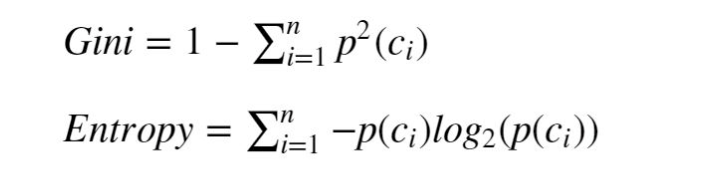
As a result of the likelihood to randomly choose a pattern from class ci is p(ci). Having picked that, the likelihood to foretell the mistaken class is (1-p(ci)). If we sum p(ci)*(1-p(ci)) over all of the lessons we get the system for the Gini impurity in Fig.4.
With the Gini index as goal, the tree chooses in every step the function and threshold that cut up the inhabitants in a manner that maximally decreases the weighted common Gini of the 2 ensuing populations (or maximally enhance their weighted common homogeneity). In different phrases, the practice logic is to reduce the likelihood of random classification error within the two ensuing populations, with extra weight placed on the bigger of the sub populations.
And sure — the mechanism goes over all of the pattern values and splits them in line with the criterion to examine the ensuing Gini.
From this definition we are able to additionally perceive why the brink values are at all times precise values discovered on at the least one of many practice samples — there isn’t any acquire in utilizing a price that’s within the hole between samples for the reason that ensuing cut up could be equivalent.
One other metric that’s generally used for tree coaching is entropy (see system in Fig.4).
Entropy
Whereas the Gini technique goals to reduce the random classification error within the subsequent step, the entropy minimization technique goals to maximise the data acquire.
Data acquire
In absence of a previous information of how a inhabitants is split into 10 lessons, we assume it’s divided evenly between them. On this case, we want a median of three.3 sure/no questions to seek out out the classification of a pattern (are you class 1–5? If not — are you class 6–8? and so forth.). Because of this the entropy of the inhabitants is 3.3 bits.
however now let’s assume that we did one thing (like a intelligent cut up) that gave us data on the inhabitants distribution, and now we all know that fifty% of the samples are at school 1, 25% at school 2 and 25% of the samples at school 3. On this case the entropy of the inhabitants will probably be 1.5 — we solely want 1.5 bits to explain a random pattern. (First query — are you class 1? The sequence will finish right here 50% of the time. Second query — are you class 2? and no extra questions are required — so 50%*1 + 50%*2 = 1.5 questions on common). That data we gained is value 1.8 bits.
Like Gini, minimizing entropy can be aligned with making a extra homogeneous inhabitants, since homogeneous populations have decrease entropy (with the acute of a single-class inhabitants having a 0 entropy — no must ask any sure/no questions).
Gini or Entropy?
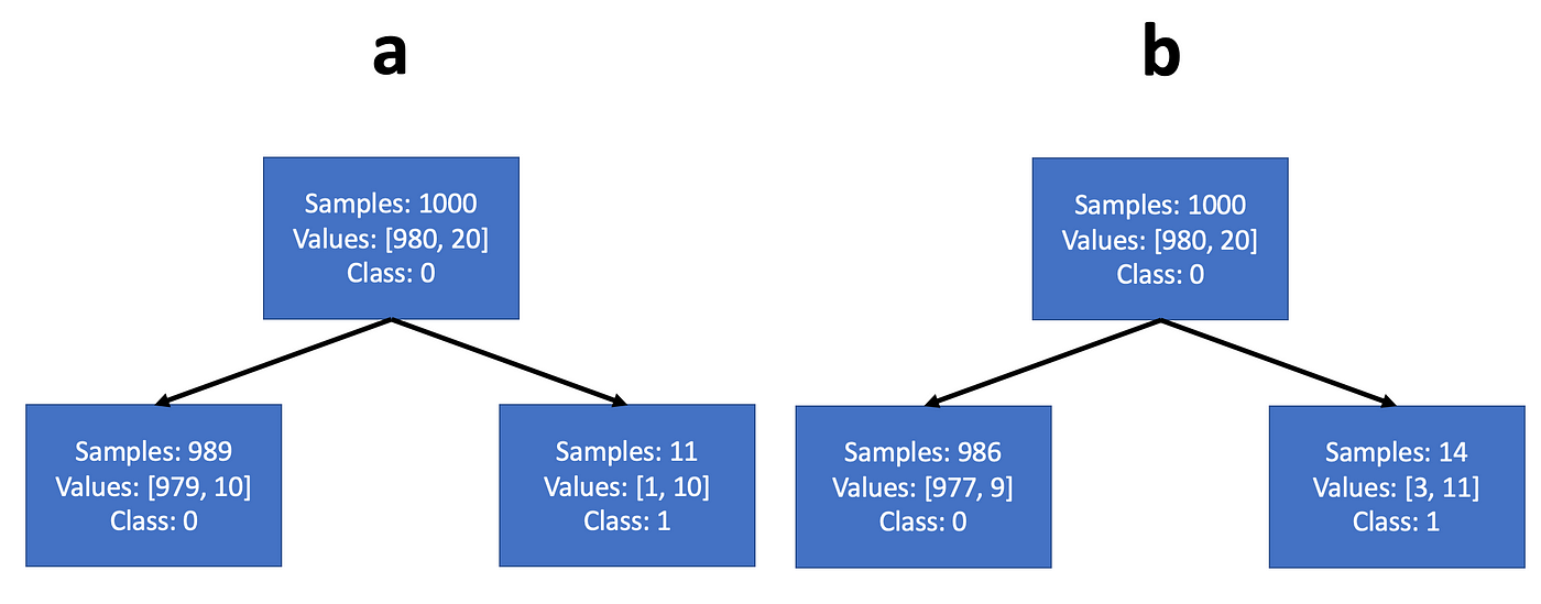
Most sources declare that the distinction between the 2 methods is just not that important (certainly — when you attempt to practice an entropy tree on the issue we simply labored — you’re going to get precisely the identical splits). It’s straightforward to see why: whereas Gini maximizes the expectation worth of a category likelihood, entropy maximizes the expectation worth of the log class likelihood. However the log likelihood is a monotonically growing perform of the likelihood, so that they often function fairly equally. Nevertheless, entropy minimization might select a distinct configuration than Gini, when the inhabitants is extremely unbalanced. For instance, we are able to consider a dataset with 1000 coaching samples — 980 belong to class 0 and 20 to class 1. Let’s say the tree can select a threshold that might cut up it both in line with instance a or instance b in Fig.5. We be aware that each examples create a node with a big inhabitants composed primarily of the bulk class, and the a second node with small inhabitants composed primarily of the minority class.
In such a case, the steepness of the log perform at small values will inspire the entropy criterion to purify the node with the big inhabitants, extra strongly than the Gini criterion. So if we work out the mathematics, we’ll see that the Gini criterion would select cut up a, and the entropy criterion would chooses cut up b.
This may occasionally result in a distinct alternative of function/threshold. Not essentially higher or worse — this will depend on our objectives.
Notice that even in issues with initially balanced populations, the decrease nodes of the classification tree will sometimes have extremely unbalanced populations.
When a path within the tree reaches the required depth worth, or when it accommodates a zero Gini/entropy inhabitants, it stops coaching. When all of the paths stopped coaching, the tree is prepared.
A typical apply is to restrict the depth of a tree. One other is to restrict the variety of samples in a leaf (not permitting fewer samples than a threshold). Each practices are accomplished to forestall overfitting on the practice set.
Now that we’ve labored out the small print on coaching a classification tree, will probably be very easy to know regression timber: The labels in regression issues are steady reasonably than discrete (e.g. the effectiveness of a given drug dose, measured in % of the circumstances). Coaching on one of these drawback, regression timber additionally classify, however the labels are dynamically calculated because the imply worth of the samples in every node. Right here, it is not uncommon to make use of imply sq. error or Chi sq. measure as targets for minimization, as an alternative of Gini and entropy.
On this publish we realized that call timber are principally comparability sequences that may practice to carry out classification and regression duties. We ran python scripts that educated a choice tree classifier, used our classifier to foretell the category of a number of information samples, and computed the precision and recall metrics of the predictions on the coaching set and the take a look at set. We additionally realized the mathematical mechanism behind the choice tree coaching, that goals to reduce some prediction error metric (Gini, entropy, mse) after every comparability. I hope you loved studying this publish, see you in my different posts!
