A whole Python implementation and clarification of the calculations behind measuring characteristic significance in tree-based machine studying algorithms
The purpose of this text is to familiarize the reader with how are the significance of options calculated in determination bushes. Personally, I’ve not discovered an in-depth clarification of this idea and thus this text was born.
All of the code used on this article is publicly out there and will be discovered by way of:
Earlier than diving deeper into the characteristic significance calculation, I extremely suggest refreshing your information about what a tree is and the way can we mix them right into a random forest utilizing these articles:
We are going to use a choice tree mannequin to create a relationship between the median home value (Y) in California utilizing numerous regressors (X). The dataset¹ will be loaded utilizing the scikit-learn package deal:
The options X that we’ll use within the fashions are:
* MedInc — Median family revenue previously 12 months (lots of of 1000’s)
* HouseAge — Age of the home (years)
* AveRooms — Common variety of rooms per dwelling
* AveBedrms — Common variety of bedrooms per dwelling
* AveOccup — Common variety of family members
The response variable Y is the median home worth for California districts, expressed in lots of of 1000’s of {dollars}.
The form of the info is the next:

Fast look on the characteristic variables:


Distribution of the Y variable:
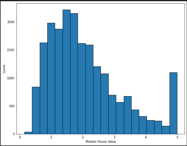
With a view to anonymize the info, there’s a cap of 500 000$ revenue within the information: something above it’s nonetheless labelled as 500 000$ revenue. That is to make sure that no individual can establish the precise family as a result of again in 1997 there weren’t many households that have been this costly.
We are going to break up the info right into a coaching and take a look at set, match a regression tree mannequin and infer the outcomes each on the coaching set and on the take a look at set.
The printouts are:

The grown tree doesn’t overfit. This text is in regards to the inference of options, so we is not going to strive our greatest to scale back the errors however relatively attempt to infer which options have been essentially the most influential ones.
The total-grown tree on the coaching set:

A choice tree is made up of nodes, every linked by a splitting rule. The splitting rule entails a characteristic and the worth it must be break up on.
The time period break up implies that if the splitting rule is happy, an commentary from the dataset goes to the left of the node. If the rule is just not happy, the commentary goes to the precise.
Every node is enumerated from 1 to fifteen.
Allow us to study the primary node and the data in it. The logic for all of the nodes would be the similar.
MedInc ≤ 5.029 — the splitting rule of the node. If an commentary has the MedInc worth much less or equal to five.029, then we traverse the tree to the left (go to node 2), in any other case, we go to the precise node (node quantity 3).
squared_error — the statistic that’s used because the splitting standards. The squared_error is calculated with the next method:
Within the first node, the statistic is the same as 1.335.
samples — the variety of observations within the node. As a result of that is the basis node, 15480 corresponds to the entire coaching dataset.
worth — the expected worth of the node. In different phrases, if the commentary path stops at this node, then the expected worth for that node could be 2.074.
Allow us to create a dictionary that holds all of the observations in all of the nodes:
n_entries = {
“node 1”: 15480,
“node 2”: 12163,
“node 3”: 3317,
“node 4”: 5869,
“node 5”: 6294,
“node 6”: 2317,
“node 7”: 1000,
“node 8”: 2454,
“node 9”: 3415,
“node 10”: 1372,
“node 11”: 4922,
“node 12”: 958,
“node 13”: 1359,
“node 14”: 423,
“node 15”: 577
}
When calculating the characteristic importances, one of many metrics used is the chance of commentary to fall right into a sure node. The chance is calculated for every node within the determination tree and is calculated simply by dividing the variety of samples within the node by the whole quantity of observations within the dataset (15480 in our case).
Allow us to denote that dictionary as n_entries_weighted:
n_entries_weighted = {
'node 1': 1.0,
'node 2': 0.786,
'node 3': 0.214,
'node 4': 0.379,
'node 5': 0.407,
'node 6': 0.15,
'node 7': 0.065,
'node 8': 0.159,
'node 9': 0.221,
'node 10': 0.089,
'node 11': 0.318,
'node 12': 0.062,
'node 13': 0.088,
'node 14': 0.027,
'node 15': 0.037
}
To place some mathematical rigour into the definition of the characteristic importances, allow us to use mathematical notations within the textual content.
Allow us to denote every node as
Every node, up till the ultimate depth, has a left and a proper youngster. Let’s denote them as:
Every node has sure properties. Allow us to denote the weights we simply calculated within the earlier part as:
Allow us to denote the imply squared error (MSE) statistic as:
One crucial attribute of a node that has kids is the so-called node significance:
The above equation’s instinct is that if the MSE within the kids is small, then the significance of the node and particularly its splitting rule characteristic is large.
Allow us to create a dictionary with every node’s MSE statistic:
i_sq = {
“node 1”: 1.335,
“node 2”: 0.832,
“node 3”: 1.214,
“node 4”: 0.546,
“node 5”: 0.834,
“node 6”: 0.893,
“node 7”: 0.776,
“node 8”: 0.648,
“node 9”: 0.385,
“node 10”: 1.287,
“node 11”: 0.516,
“node 12”: 0.989,
“node 13”: 0.536,
“node 14”: 0.773,
“node 15”: 0.432
}
Authors Trevor Hastie, Robert Tibshirani and Jerome Friedman of their nice guide The Components of Statistical Studying: Knowledge Mining, Inference, and Prediction outline the characteristic significance calculation with the next equation²:
The place
T — is the entire determination tree
l — characteristic in query
J — variety of inner nodes within the determination tree
i² — the discount within the metric used for splitting
II — indicator operate
v(t) — a characteristic utilized in splitting of the node t utilized in splitting of the node
The instinct behind this equation is, to sum up all of the decreases within the metric for all of the options throughout the tree.
Scikit-learn makes use of the node significance method proposed earlier. The primary distinction is that in scikit-learn, the node weights are launched which is the chance of an commentary falling into the tree.
Allow us to zoom in somewhat bit and examine nodes 1 to three a bit additional.

The calculation of node significance (and thus characteristic significance) takes one node at a time. The following logic defined for node #1 holds for all of the nodes right down to the degrees beneath.
Solely nodes with a splitting rule contribute to the characteristic significance calculation.
The 2nd node is the left youngster and the third node is the precise youngster of node #1.
The instinct behind characteristic significance begins with the concept of the whole discount within the splitting standards. In different phrases, we need to measure, how a given characteristic and its splitting worth (though the worth itself is just not used wherever) scale back the, in our case, imply squared error within the system. The node significance equation outlined within the part above captures this impact.
If we use MedInc within the root node, there will probably be 12163 observations going to the second node and 3317 going to the precise node. This interprets to the load of the left node being 0.786 (12163/15480) and the load of the precise node being 0.214 (3317/15480). The imply squared error within the left node is the same as 0.892 and in the precise node, it is 1.214.
We have to calculate the node significance:
Now we are able to save the node significance right into a dictionary. The dictionary keys are the options which have been used within the node’s splitting standards. The values are the node’s significance.
{
"MedInc": 0.421252,
"HouseAge": 0,
"AveRooms": 0,
"AveBedrms": 0,
"AveOccup": 0}
The above calculation process must be repeated for all of the nodes with a splitting rule.
Allow us to do a couple of extra node calculations to fully get the dangle of the algorithm:

The squared error if we use the MedInc characteristic in node 2 is:
The characteristic significance dictionary now turns into:
{
"MedInc": 0.421 + 0.10758
"HouseAge": 0,
"AveRooms": 0,
"AveBedrms": 0,
"AveOccup": 0}

{
"MedInc": 0.558,
"HouseAge": 0,
"AveRooms": 0.018817,
"AveBedrms": 0,
"AveOccup": 0}
We can’t go any additional, as a result of nodes 8 and 9 wouldn’t have a splitting rule and thus don’t additional scale back the imply squared error statistic.
Allow us to code up the implementation that was introduced within the sections above.
Now let’s outline a operate that calculates the node’s significance.
Placing all of it collectively:
The prints within the above code snippet are:
Node significance: {
‘node 1’: 0.421,
‘node 2’: 0.108,
‘node 3’: 0.076,
‘node 4’: 0.019,
‘node 5’: 0.061,
‘node 6’: 0.025,
‘node 7’: 0.013
} Characteristic significance earlier than normalization: {
‘MedInc’: 0.618,
‘AveRooms’: 0.019,
‘AveOccup’: 0.086,
‘HouseAge’: 0,
‘AveBedrms’: 0
} Characteristic significance after normalization: {
‘MedInc’: 0.855,
‘AveRooms’: 0.026,
‘AveOccup’: 0.119,
‘HouseAge’: 0.0,
‘AveBedrms’: 0.0
}
The ultimate characteristic dictionary after normalization is the dictionary with the ultimate characteristic significance. In response to the dictionary, by far crucial characteristic is MedInc adopted by AveOccup and AveRooms.
The options HouseAge and AveBedrms weren’t utilized in any of the splitting guidelines and thus their significance is 0.
Allow us to evaluate our calculation with the scikit-learn implementation of characteristic significance calculation.
The print reads:
Characteristic significance by sklearn:
{
‘MedInc’: 0.854,
‘HouseAge’: 0.0,
‘AveRooms’: 0.027,
‘AveBedrms’: 0.0,
‘AveOccup’: 0.12
}
Evaluating it with our calculations:

There are minimal variations, however these are resulting from rounding errors.
On this article, I’ve demonstrated the characteristic significance calculation in nice element for determination bushes. A really related logic applies to determination bushes utilized in classification. The one distinction is the metric — as a substitute of utilizing squared error, we use the GINI impurity metric (or different classification evaluating metric). All of the calculations concerning node significance keep the identical.
I hope that after studying all this you’ll have a a lot clearer image of learn how to interpret and the way the calculations are made concerning characteristic significance.
Pleased coding!
[1] Creator: Tempo, R. Kelley and Ronald Barry
Yr: 1997
Title: Sparse Spatial Autoregressions
URL: http://archive.ics.uci.edu/ml
Journal: Statistics and Chance Letters
[2] Creator: Trevor Hastie, Robert Tibshirani and Jerome Friedman
Yr: 2017
Title: The Components of Statistical Studying: Knowledge Mining, Inference, and Prediction
URL: http://archive.ics.uci.edu/ml
Web page: 368–370
