Bettering Advertising and marketing Combine Modeling Utilizing Machine Studying Approaches | by Slava Kisilevich | Jun, 2022

Constructing MMM fashions utilizing tree-based ensembles and explaining media channel efficiency utilizing SHAP (Shapley Additive Explanations)

Tlisted here are some ways one can construct a advertising combine mannequin (MMM) however normally, it boils all the way down to utilizing linear regression for its easy interpretability. Interpretability of extra complicated non-linear fashions is the subject of analysis within the final 5–6 years since such ideas as LIME or SHAP had been proposed within the machine studying group to clarify the output of a mannequin. Nonetheless, these new ideas appear to be virtually unknown within the subject of selling attribution. On this article, I proceed investigating sensible approaches in advertising combine modeling by constructing tree-based ensembles utilizing Random Forest and explaining media channel efficiency utilizing the SHAP idea.

In my earlier article, I used bayesian programming to construct a advertising combine mannequin and in contrast the outcomes to the Robyn framework. My major curiosity was to analyze if each approaches are comparable and could be constant in storytelling. Since Robyn generates a number of options, I used to be capable of finding the one, which is in keeping with the Bayesian resolution, particularly that shares of results of each fashions are constantly increased or decrease than shares of spending in every channel. The share variations may very well be attributed to variations in approaches and the flexibility of fashions to suit the info effectively. Nonetheless, the widespread between the 2 approaches is that each describe a linear relationship between media spending and response and are therefore unable to seize extra complicated variable relationships corresponding to interactions.

One of many first business proof of ideas for utilizing extra complicated algorithms like Gradient Boosting Machines (GBM) together with SHAP in advertising combine modeling, that I may discover, was described by H2O.ai.

I summarise the principle motivations behind switching to extra complicated algorithms:

• Classical approaches like linear regression, are difficult and require time and experience to establish correct mannequin constructions corresponding to variable correlations, interactions, or non-linear relationships. In some instances, extremely correlated options must be eliminated. Interplay variables must be explicitly engineered. Non-linearities like saturation and diminishing returns must be explicitly launched by totally different transformations.
• Some mannequin constructions are sacrificed for the sake of simpler mannequin interpretability which can result in poor mannequin efficiency.
• Extra complicated machine studying algorithms like tree-based ensembles work effectively within the presence of extremely correlated variables, could seize interactions between variables, are non-linear, and are normally extra correct.

The main points behind SHAP for mannequin rationalization are defined in lots of articles and books. I summarise the principle instinct behind SHAP beneath:

SHAP (SHapley Additive exPlanations) is a recreation theoretic method to clarify the output of any machine studying mannequin. It connects optimum credit score allocation with native explanations utilizing the traditional Shapley values from recreation idea and their associated extensions

• SHAP is a technique for explaining particular person predictions and solutions the query of how a lot does every function contribute to this prediction
• SHAP values are measures of function significance
• SHAP values could be destructive and optimistic and present the magnitude of prediction relative to the typical of all predictions. Absolutely the magnitude signifies the energy of the function for a specific particular person prediction
• The common of absolute magnitudes of SHAP values per function signifies the worldwide significance of the function
• Not directly, SHAP function significance could be various to permutation function significance. In distinction to SHAP, permutation function significance is predicated on an general lower in mannequin efficiency.

The most important problem in switching to extra complicated fashions in MMM was the dearth of instruments to clarify the affect of particular person media channels. Whereas the machine studying group is extensively utilizing approaches for mannequin explainability like SHAP, which is usually recommended by tons of of papers and convention talks, it’s nonetheless very troublesome to seek out examples of SHAP utilization within the MMM context. This nice article connects MMM with SHAP and explains how we could interpret the outcomes of the advertising combine. Motivated by this text, I wrote an virtually generic resolution to mannequin a advertising combine, by combining concepts of Robyn’s methodology for pattern and seasonality decomposition, utilizing a Random Forest estimator (which could be simply modified to different algorithms), and optimizing adstock and model-specific parameters utilizing Optuna (hyperparameter optimization framework). The answer permits switching between single goal optimization as is normally performed in MMM and a number of goal optimization as is finished by Robyn.

I proceed utilizing the dataset made accessible by Robyn below MIT Licence as in my first article for consistency and benchmarking, and comply with the identical information preparation steps by making use of Prophet to decompose developments, seasonality, and holidays.

The dataset consists of 208 weeks of income (from 2015–11–23 to 2019–11–11) having:

• 5 media spend channels: tv_S, ooh_S, print_S, facebook_S, search_S
• 2 media channels which have additionally the publicity info (Impression, Clicks): facebook_I, search_clicks_P (not used on this article)
• Natural media with out spend: e-newsletter
• Management variables: occasions, holidays, competitor gross sales (competitor_sales_B)

The evaluation window is 92 weeks from 2016–11–21 to 2018–08–20.

Regardless of a modeling algorithm, the promoting adstock performs an essential function in MMM. Subsequently, we have now to determine what sort of adstock we’re going to experiment with and what are the minimal and most values it could probably have for every media channel (please check with my earlier article for an outline of varied adstock capabilities). The optimization algorithm will attempt every adstock worth from the vary of outlined values to seek out the perfect one which minimizes the optimization standards.

I’m utilizing the geometric adstock perform applied in scikit-learn as follows:

from sklearn.base import BaseEstimator, TransformerMixin
from sklearn.utils import check_array
from sklearn.utils.validation import check_is_fittedclass AdstockGeometric(BaseEstimator, TransformerMixin):
def __init__(self, alpha=0.5):
self.alpha = alpha
def match(self, X, y=None):
X = check_array(X)
self._check_n_features(X, reset=True)
return self
def remodel(self, X: np.ndarray):
check_is_fitted(self)
X = check_array(X)
self._check_n_features(X, reset=False)
x_decayed = np.zeros_like(X)
x_decayed[0] = X[0]
for xi in vary(1, len(x_decayed)):
x_decayed[xi] = X[xi] + self.alpha* x_decayed[xi - 1]
return x_decayed

I already talked about that linear fashions aren’t capable of seize the non-linear relationships between totally different ranges of commercial spending and the end result. Subsequently, numerous non-linear transformations corresponding to Energy, Detrimental Exponential, and Hill had been utilized to media channels previous to modeling.

Tree-based algorithms are capable of seize non-linearities. Subsequently, I don’t apply any non-linear transformation explicitly and let the mannequin be taught non-linearities by itself.

Modeling consists of a number of steps:

Adstock parameters

How lengthy the advert could have an impact is dependent upon the media channel. Since we’re looking for an optimum adstock decay charge, we have now to be practical concerning the potential ranges of the parameter. For instance, it’s recognized {that a} TV commercial could have a long-lasting impact whereas Print has a shorter impact. So we have now to have the flexibleness of defining practical hyperparameters for every media channel. On this instance, I’m utilizing the precise ranges proposed by Robyn of their demo file.

adstock_features_params = {}
adstock_features_params["tv_S_adstock"] = (0.3, 0.8)
adstock_features_params["ooh_S_adstock"] = (0.1, 0.4)
adstock_features_params["print_S_adstock"] = (0.1, 0.4)
adstock_features_params["facebook_S_adstock"] = (0.0, 0.4)
adstock_features_params["search_S_adstock"] = (0.0, 0.3)
adstock_features_params["newsletter_adstock"] = (0.1, 0.4)

Time Collection Cross-Validation

We wish to discover parameters that generalize effectively to unseen information. We’ve to separate our information right into a coaching and check set. Since our information represents spending and revenues occurring alongside the timeline we have now to use a time sequence cross-validation such that the coaching set consists solely of occasions that occurred previous to occasions within the check set.

Machine studying algorithms work greatest when they’re educated on massive quantities of information. The Random Forest algorithm shouldn’t be an exception and so as to seize non-linearities and interactions between variables, it must be educated on lots of information. As I discussed earlier, we have now solely 208 information factors in whole and 92 information factors within the evaluation window. We want some trade-off between generalizability and the potential of a mannequin to be taught.

After some experiments, I made a decision to make use of 3 cv-splits by allocating 20 weeks of information (about 10%) as a check set.

from sklearn.model_selection import TimeSeriesSplit
tscv = TimeSeriesSplit(n_splits=3, test_size = 20)

Every successive coaching set break up is bigger than the earlier one.

tscv = TimeSeriesSplit(n_splits=3, test_size = 20)
for train_index, test_index in tscv.break up(information):
print(f"prepare measurement: {len(train_index)}, check measurement: {len(test_index)}")#prepare measurement: 148, check measurement: 20
#prepare measurement: 168, check measurement: 20
#prepare measurement: 188, check measurement: 20

Hyperparameter optimization utilizing Optuna

Hyperparameter optimization consists of quite a lot of experiments or trials. Every trial could be roughly divided into three steps.

• Apply adstock transformation on media channels utilizing a set of adstock parameters

for function in adstock_features:
adstock_param = f"{function}_adstock"
min_, max_ = adstock_features_params[adstock_param]
adstock_alpha = trial.suggest_uniform(f"adstock_alpha_{function}", min_, max_)
adstock_alphas[feature] = adstock_alpha
#adstock transformation
x_feature = information[feature].values.reshape(-1, 1)
temp_adstock = AdstockGeometric(alpha = adstock_alpha).fit_transform(x_feature)
data_temp[feature] = temp_adstock

#Random Forest parameters
n_estimators = trial.suggest_int("n_estimators", 5, 100)
min_samples_leaf = trial.suggest_int('min_samples_leaf', 1, 20)
min_samples_split = trial.suggest_int('min_samples_split', 2, 20)
max_depth = trial.suggest_int("max_depth", 4,7)
ccp_alpha = trial.suggest_uniform("ccp_alpha", 0, 0.3)
bootstrap = trial.suggest_categorical("bootstrap", [False, True])
criterion = trial.suggest_categorical("criterion",["squared_error"])

• Cross-validate and measure the typical error throughout all check units

for train_index, test_index in tscv.break up(data_temp):
x_train = data_temp.iloc[train_index][features]
y_train =  data_temp[target].values[train_index]
x_test = data_temp.iloc[test_index][features]
y_test = data_temp[target].values[test_index]
#apply Random Forest
params = {"n_estimators": n_estimators, 
"min_samples_leaf":min_samples_leaf, 
"min_samples_split" : min_samples_split,
"max_depth" : max_depth, 
"ccp_alpha" : ccp_alpha, 
"bootstrap" : bootstrap, 
"criterion" : criterion
}
#prepare a mannequin      
rf = RandomForestRegressor(random_state=0, **params)
rf.match(x_train, y_train)
#predict check set
prediction = rf.predict(x_test)
#RMSE error metric       
rmse = mean_squared_error(y_true = y_test, y_pred = prediction, squared = False)
#accumulate errors for every fold
scores.append(rmse)#lastly return the typical of the cv error
return np.imply(scores)

Every trial returns the adstock, mannequin parameters, and error metrics as a person attribute. This enables straightforward retrieval of the parameters in the perfect trial.

trial.set_user_attr("scores", scores)
trial.set_user_attr("params", params)
trial.set_user_attr("adstock_alphas", adstock_alphas)

The primary perform to begin the optimization is optuna_optimize. It returns the Optuna Examine object with all trials together with the perfect trial (having a minimal common RMSE error)

tscv = TimeSeriesSplit(n_splits=3, test_size = 20)adstock_features_params = {}
adstock_features_params["tv_S_adstock"] = (0.3, 0.8)
adstock_features_params["ooh_S_adstock"] = (0.1, 0.4)
adstock_features_params["print_S_adstock"] = (0.1, 0.4)
adstock_features_params["facebook_S_adstock"] = (0.0, 0.4)
adstock_features_params["search_S_adstock"] = (0.0, 0.3)
adstock_features_params["newsletter_adstock"] = (0.1, 0.4)OPTUNA_TRIALS = 2000#experiment is an optuna research object
experiment = optuna_optimize(trials = OPTUNA_TRIALS, 
information = information, 
goal = goal, 
options = options, 
adstock_features = media_channels + organic_channels, 
adstock_features_params = adstock_features_params, 
media_features=media_channels, 
tscv = tscv, 
is_multiobjective=False)

RMSE rating for every fold of the perfect trial:

experiment.best_trial.user_attrs["scores"]#[162390.01010327024, 114089.35799374945, 79415.8649240292]

Adstock parameters akin to the perfect trial:

experiment.best_trial.user_attrs["adstock_alphas"]#{'tv_S': 0.5343389820427953,
# 'ooh_S': 0.21179063584028718,
# 'print_S': 0.27877433150946473,
# 'facebook_S': 0.3447366707231967,
# 'search_S': 0.11609804659096469,
# 'e-newsletter': 0.2559060243894163}

Mannequin parameters akin to the perfect trial:

experiment.best_trial.user_attrs["params"]#{'n_estimators': 17,
# 'min_samples_leaf': 2,
# 'min_samples_split': 4,
# 'max_depth': 7,
# 'ccp_alpha': 0.19951653203058856,
# 'bootstrap': True,
# 'criterion': 'squared_error'}

Last Mannequin

I construct the ultimate mannequin utilizing the optimized parameters by offering the beginning and finish intervals for evaluation. The mannequin is first constructed on all the info as much as the tip of the evaluation interval. The predictions and SHAP values are retrieved for the evaluation interval solely.

best_params = experiment.best_trial.user_attrs["params"]
adstock_params = experiment.best_trial.user_attrs["adstock_alphas"]
end result = model_refit(information = information, 
goal = goal,
options = options, 
media_channels = media_channels, 
organic_channels = organic_channels, 
model_params = best_params, 
adstock_params = adstock_params, 
start_index = START_ANALYSIS_INDEX, 
end_index = END_ANALYSIS_INDEX)

The primary plot to verify is how effectively the mannequin matches the info for the evaluation interval of 92 weeks:

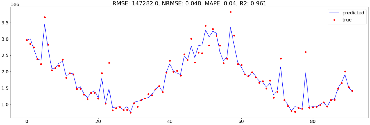
MAPE improved by 40% and NRMSE by 17% in comparison with the Bayesian method.

Subsequent, let’s plot the share of spend vs. share of impact:

The share of impact is calculated utilizing absolutely the sum of SHAP values for every media channel throughout the evaluation interval and normalized by the overall sum of SHAP values of all media channels.

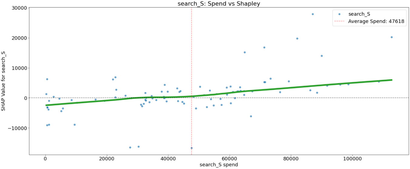
The share of impact is nearly in keeping with the share of impact of the earlier article. I observe just one inconsistency between the share of impact of the search channel.

Diminishing return / Saturation impact

I didn’t apply any non-linear transformations to explicitly mannequin the diminishing returns. So let’s verify if Random Forest may seize any non-linearities.

That is achieved by the scatter plot that reveals the impact a single media channel has on the predictions made by the mannequin the place the x-axis is the media spend, the y-axis is the SHAP worth for that media channel, which represents how a lot understanding a specific spend modifications the output of the mannequin for that specific prediction. The horizontal line corresponds to the SHAP worth of 0. The vertical line corresponds to the typical spend within the channel. The inexperienced line is a LOWESS smoothing curve.

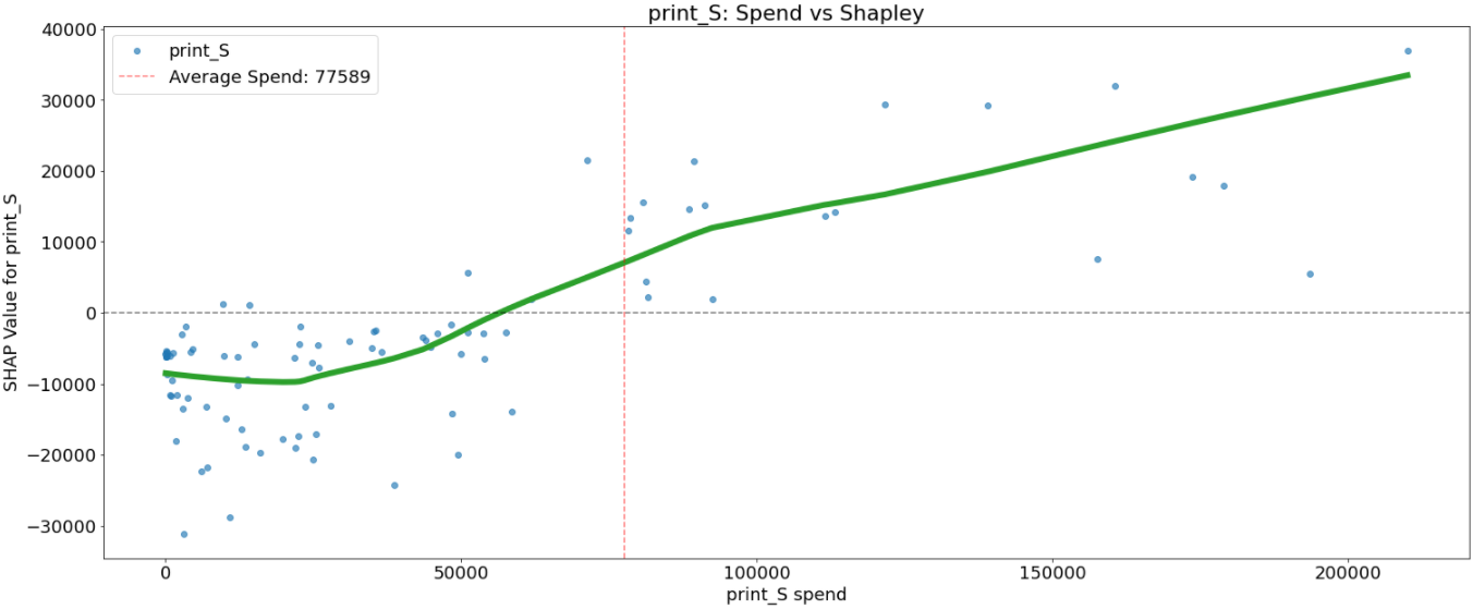
all media channels, we will see that increased spend is related to a rise in income. However the relations aren’t all the time linear.

Taking print_S we will observe a slight lower in income for spend as much as 25K. Then it begins to extend as much as about 90K the place the rise in income is slowed down.

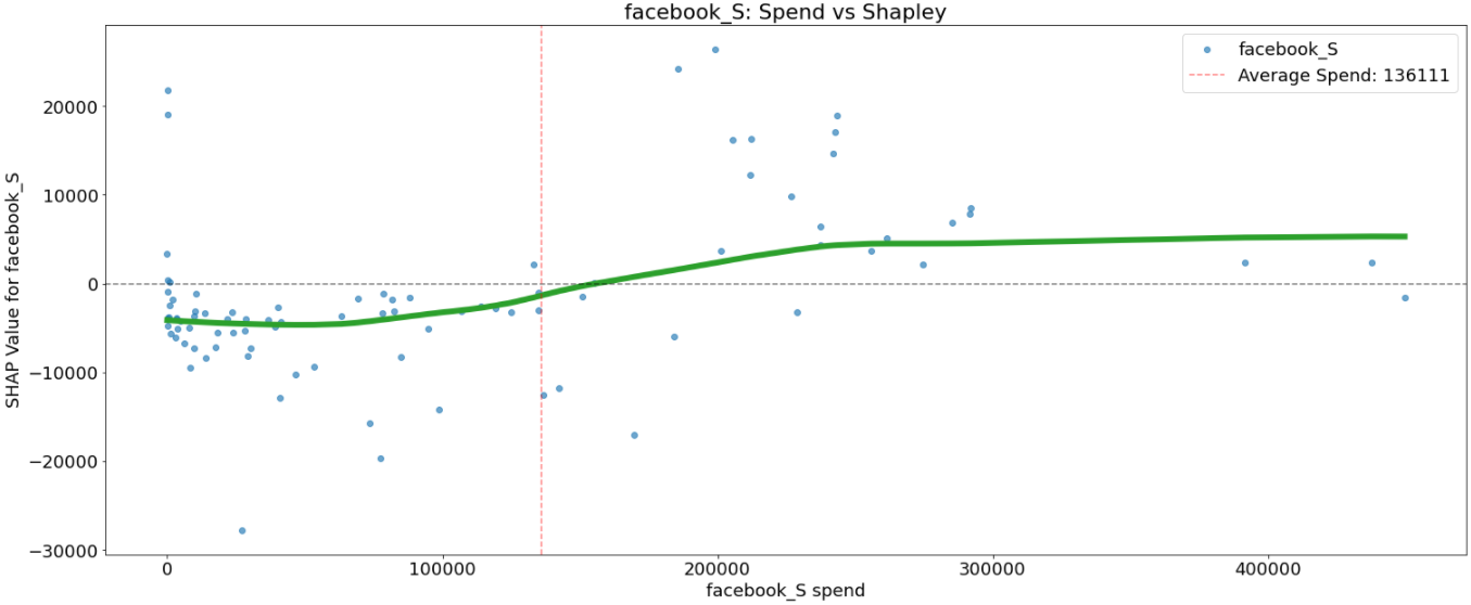
Taking facebook_S we will observe virtually no change in income for spend as much as 90K and after 250K. Spends between 90K and 250K are in all probability probably the most optimum spending.

Some media channels like facebook_S, print_S, and search_S have a excessive variance between SHAP values for a similar spend. This may be defined by interplay with different media channels and must be additional investigated.

This resolution can handle multiobjective optimization. The concept comes from Robyn by introducing a second optimization metric RSSD (decomposition root-sum-square distance)

The space accounts for a relationship between spend share and a channel’s coefficient decomposition share. If the space is just too far, its end result could be too unrealistic — e.g. media exercise with the smallest spending will get the most important impact

Within the case of multiobjective optimization, the so-called Pareto Entrance, the set of all optimum options, will probably be decided by Optuna. The process would be the identical as for a single optimization case: for every mannequin belonging to the Pareto Entrance, we retrieve its parameters, construct a remaining mannequin and visualize the outcomes.
Within the graph beneath all factors with the reddish shade belong to the optimum set.

On this article, I continued exploring methods to enhance fashions for Advertising and marketing Combine through the use of extra complicated algorithms which can be capable of seize non-linearities and variable interactions. Consequently, the entire pipeline is simplified by omitting the non-linear transformation step, which is all the time utilized when utilizing linear regression. Utilization of SHAP values allowed additional evaluation of impact share and response curves. My second objective was to achieve constant outcomes between totally different approaches. The comparability between the outcomes of the earlier article during which I used Bayesian modeling and the outcomes of this text confirmed a excessive diploma of consistency within the decomposed results per media channel.

The whole code could be downloaded from my Github repo

Thanks for studying!