(Be aware: this isn’t a 343 minute learn.)
Similar to each different scientist, engineer, or Matt, I’m fairly into mountain climbing. Being carless in NYC, I primarily climb indoors. One of many first issues that you simply study when going to a climbing fitness center is that you simply don’t get to seize on to each “maintain” (the brilliant plastic issues on the wall). Totally different coloured holds correspond to completely different “routes”, and also you problem your self by solely utilizing the holds for a selected route.

Embarrassingly, the one image I’ve of myself climbing is on autobelay.
How a lot do you problem your self? Effectively, that will depend on the route. Every route has a “grade” or “ranking” which describes the route’s issue. Within the US, routes that require a security rope use the Yosemite Decimal System (Supply).
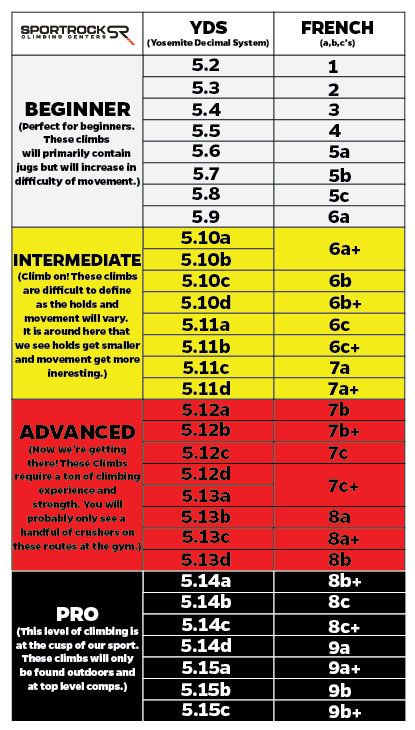
For bouldering issues (routes which are quick and fast and don’t require a rope), there’s a separate, “V-scale” US ranking system.
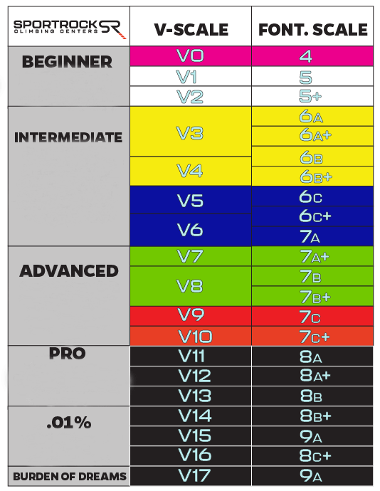
In abstract, for each climbing routes and bouldering issues, there are ranking programs the place the rise within the numerical ranking corresponds to a rise in issue. How are these rankings determined?
They’re simply made up.
This type of blew me away after I first began climbing. I assumed that you’d be required to do sure forms of strikes for sure rankings. In observe, route setters place the holds for a brand new route, they’ve a basic thought of how exhausting they assume the route is, after which they’ve a pair different folks climb it and provides their opinion.
Naturally, this bought me considering:
If I had a dataset of which routes folks had been and weren’t in a position to climb, might I mannequin a extra goal rankings system?
In all probability?
Sadly, I wouldn’t have that dataset.
I did discover one thing shut, although, and I used to be then in a position to construct some type of mannequin. Within the spirit of George Field, I constructed a mannequin that’s most undoubtedly incorrect, however it could be helpful. If nothing else, I’m hoping this mannequin will function mild introduction to Bayesian modeling in Stan.
When Folks Inform You What They’ve Performed, Imagine Them
In looking for a dataset of tried climbs, I stumbled upon this Kaggle dataset. The person who uploaded the dataset had scraped the web site www.8a.nu which is a web site the place customers can log outside climbing routes that they’ve efficiently climbed. That is the primary subject with the information: it solely accommodates profitable routes that customers have climbed. As a significant comfort, the customers do log whether or not or not they climbed the route on their first strive (aka they “flashed” the route in climber parlance). This piece of data provides me the end result variable I must construct a mannequin!
The dataset consists of a SQLite database with 4 tables containing all types of details about the routes and the customers who tried them. All informed, there are nearly 5 million logged climbs from nearly 67K customers.
Let’s go forward and cargo the information right into a Pandas DataFrame. To maintain issues manageable, we’ll restrict to climbs within the USA.
%config InlineBackend.figure_format = 'retina'
import datetime as dt
import pickle
import sqlite3

import altair as alt
import arviz as az
import cycler
import matplotlib.pyplot as plt
import nest_asyncio
import numpy as np
import pandas as pd
from scipy.stats import gaussian_kde
# Required earlier than importing stan in a jupyter pocket book.
nest_asyncio.apply()
/dwelling/er/.pyenv/variations/route-response/lib/python3.9/site-packages/setuptools/distutils_patch.py:25: UserWarning: Distutils was imported earlier than Setuptools. This utilization is discouraged and should exhibit undesirable behaviors or errors. Please use Setuptools' objects straight or at the least import Setuptools first.
  warnings.warn(
pd.set_option("show.max_columns", None)
# Whether or not or to not use the mannequin that is already been fitted.
USE_CACHE = True
conn = sqlite3.join("database.sqlite")
question = """
SELECT
  ascent.user_id
  , ascent.crag
  , ascent.climb_type
  , ascent.title AS route_name
  , ascent.date AS ascent_date
  , REPLACE(ascent.crag, ' ', '_')
      || '__' || REPLACE(ascent.title, ' ', '_')
      || '__' || CASE WHEN ascent.climb_type = 1 THEN 'boulder' ELSE 'rope' END
      AS route_id
  , grade.usa_routes
  , grade.usa_boulders
  , technique.title AS method_name
FROM ascent
JOIN grade ON grade.id = ascent.grade_id
JOIN technique ON technique.id = ascent.method_id
WHERE
  ascent.nation = 'USA'
"""
df = pd.read_sql_query(question, conn)
      user_id
      crag
      climb_type
      route_name
      ascent_date
      route_id
      usa_routes
      usa_boulders
      method_name


      0
      25
      Hueco Tanks
      1
      Frogger
      917823600
      Hueco_Tanks__Frogger__boulder
      5.12d
      V9
      Redpoint


      1
      25
      Hueco Tanks
      1
      Intercourse After Loss of life
      917823600
      Hueco_Tanks__Sex_After_Death__boulder
      5.12d
      V9
      Redpoint


      2
      25
      Hueco Tanks
      1
      Crimson
      915145200
      Hueco_Tanks__Red__boulder
      5.12d
      V9
      Redpoint


      3
      25
      Hueco Tanks
      1
      Higher Eat Your Wheaties
      949359600
      Hueco_Tanks__Better_Eat_Your_Wheaties__boulder
      5.12c
      V8/9
      Redpoint


      4
      25
      Horse Flats
      1
      Clean Era
      957132000
      Horse_Flats__Blank_Generation__boulder
      5.12d
      V9
      Redpoint
Every row within the above desk corresponds to an ascent by a person. The crag refers back to the space the place the route is positioned. The climb_type is 1 if it’s a bouldering route, and 0 if it’s a rope route. The ascent_date is in Unix time. usa_routes and usa_boulders seek advice from the person’s ranking of the route. For some motive, many routes have each a rope and bouldering ranking. Lastly, method_name corresponds to “how” the person climbed the route. Choices embody:
Onsight: The person climbed the route on their first strive with out figuring out something in regards to the route.Flash: The person climbed the route on their first strive, however they’d studied the route forward of time.Redpoint: The person efficiently climbed the route after a number of makes an attempt.Toprope: The person climbed the route prime rope slightly than lead model (prime roping is less complicated).
Lastly, I’ve created a singular route_id for every route which is a mix of the crag, the route_name, and climb_type.
Let’s go forward and create some derived columns from the information. To start out, we’d prefer to assign a single route_rating and bouldering_grade to every route, slightly than every person specifying their very own ranking. We’ll decide the one rankings by assigning the preferred person ranking.
# Repair dtypes
def cast_columns(
    df: pd.DataFrame,
    route_ratings: pd.CategoricalDtype,
    bouldering_grades: pd.CategoricalDtype,
) -> pd.DataFrame:
    # Repair dtypes
    df["ascent_date"] = pd.to_datetime(df["ascent_date"], unit="s")
    df["usa_boulders"] = df["usa_boulders"].astype(bouldering_grades)
    df["usa_routes"] = df["usa_routes"].astype(route_ratings)
    return df
route_ratings = pd.CategoricalDtype(
    classes=[
        "5.1",
        "5.2",
        "5.3",
        "5.4",
        "5.5",
        "5.6",
        "5.7",
        "5.8",
        "5.9",
        "5.10a",
        "5.10b",
        "5.10c",
        "5.10d",
        "5.11a",
        "5.11b",
        "5.11c",
        "5.11d",
        "5.12a",
        "5.12b",
        "5.12c",
        "5.12d",
        "5.13a",
        "5.13b",
        "5.13c",
        "5.13d",
        "5.14a",
        "5.14b",
        "5.14c",
        "5.14d",
        "5.15a",
        "5.15b",
        "5.15c",
    ],
    ordered=True,
)
bouldering_grades = pd.CategoricalDtype(
    [
        "V0",
        "V1",
        "V2",
        "V3",
        "V4",
        "V5",
        "V6",
        "V7",
        "V8",
        "V9",
        "V10",
        "V11",
        "V12",
        "V13",
        "V14",
        "V15",
        "V16",
        "V17",
        "V18",
        "V19",
        "V20",
    ],
    ordered=True,
)
df = cast_columns(df, route_ratings, bouldering_grades)
# Routes may be graded in a different way by completely different folks.
# Right here, we decide the preferred grade and assign it.
route_modes = (
    df.groupby("route_id")["usa_routes"]
    .agg(lambda x: pd.Collection.mode(x).get(0))
    .to_frame()
    .rename(columns={"usa_routes": "route_rating"})
    .astype(route_ratings)
)
bouldering_modes = (
    df.groupby("route_id")["usa_boulders"]
    .agg(lambda x: pd.Collection.mode(x).get(0))
    .to_frame()
    .rename(columns={"usa_boulders": "bouldering_grade"})
    .astype(bouldering_grades)
)
# The brand new column might be `route_rating`
df = pd.merge(
    df,
    route_modes,
    how="left",
    left_on="route_id",
    right_index=True,
)
# The brand new column might be `bouldering_grade`
df = pd.merge(
    df,
    bouldering_modes,
    how="left",
    left_on="route_id",
    right_index=True,
)
Subsequent, we assign a label which is able to point out whether or not or not the person climbed the route on their first strive. It appears like 33% of ascents had been climbed on their first strive.
df["label"] = df["method_name"].isin(["Onsight", "Flash"])
Subset the information
Subsequent, let’s reduce out some knowledge in an effort to assist our downstream modeling. Some customers have logged a number of ascents for a similar route. We’ll solely maintain the primary ascent.
# Let's simply maintain the primary ascent
first_ascents = df.groupby(["user_id", "route_id"])["ascent_date"].min().to_frame()
print(f"Whole USA ascents: {len(df):,}")
df = pd.merge(df, first_ascents, on=["user_id", "route_id", "ascent_date"])
# This can be a bit lazy -- "first" is a bit ill-defined on this context.
df = df.drop_duplicates(subset=["user_id", "route_id"], maintain="first")
print(f"First USA ascents: {len(df):,}")
Whole USA ascents: 658,822
First USA ascents: 638,305
There are lots of customers who’ve solely logged a pair ascents. Likewise, there are a lot of routes which have solely be climbed by a pair customers. The dearth of knowledge for these “uncommon” customers and routes could make modeling tough. So, we’ll restrict our dataset to solely embody customers who’ve climbed at the least 20 routes and routes which were climbed by at the least 20 folks. The code to do that finally ends up being this odd iterative course of since each time we take away customers, some routes could now not have been climbed by sufficient customers, and vice versa. On the odd probability that there’s a weirdly astute reader of my weblog, they are going to discover that the beneath operate is similar to the one which I used for limiting the interactions matrix for a recommender system.
def threshold_ascents(df: pd.DataFrame, restrict: int = 5) -> pd.DataFrame:
    """
    Restrict all ascents to solely customers who've logged >= `restrict` ascents
    and solely routes which have >= `restrict` ascents.

    That is an iterative course of as a result of limiting the customers can then
    change which routes have >= `restrict` ascents. So, this operate
    alternates forwards and backwards, limiting customers after which limiting routes,
    till each stabilize.
    """
    finished = False
    df_lim = df.copy()
    print(f"Begin variety of ascents: {len(df_lim):,}.")
    whereas not finished:
        start_shape = df_lim.form

        user_mask = df_lim["user_id"].value_counts() >= restrict
        users_to_keep = user_mask[user_mask].index
        df_lim = df_lim[df_lim["user_id"].isin(users_to_keep)]

        route_mask = df_lim["route_id"].value_counts() >= restrict
        routes_to_keep = route_mask[route_mask].index
        df_lim = df_lim[df_lim["route_id"].isin(routes_to_keep)]

        end_shape = df_lim.form
        if start_shape == end_shape:
            finished = True
    print(f"Finish variety of ascents: {len(df_lim):,}.")
    return df_lim
df = threshold_ascents(df, restrict=20)
Begin variety of ascents: 638,305.
Finish variety of ascents: 232,887.
Route Response Principle
Lastly, we will construct our mannequin. Previous to doing this, although, and in step with the aforementioned similarity to suggestion programs, we should first construct mappers between the ids in our knowledge and indices in an array. Particularly, we map the route_id to a route_idx (sorry for the poor variable naming) and the user_id to a user_idx. After constructing the mappers, we use them to create new columns within the dataset.
# Create mappers between IDs and matrix indices.
# Additionally, type the IDs in order that this operation is reproducible.
route_idx_to_id = dict(enumerate(sorted(df["route_id"].distinctive())))
route_id_to_idx = {v: ok for ok, v in route_idx_to_id.gadgets()}

user_idx_to_id = dict(enumerate(sorted(df["user_id"].distinctive())))
user_id_to_idx = {v: ok for ok, v in user_idx_to_id.gadgets()}

df["route_idx"] = df["route_id"].map(route_id_to_idx)
df["user_idx"] = df["user_id"].map(user_id_to_idx)
Okay now we will do some modeling. To mannequin our customers, routes, and ascents, we’ll flip to Merchandise Response Principle (IRT). For funsies, we’ll name our scenario Route Response Principle (RRT). I first realized about IRT a pair years in the past when studying this Sew Repair weblog publish. If you happen to learn the publish, you’ll study that IRT was initially created by the Instructional Testing Service (ETS) as a solution to evaluate college students who had seen completely different issues on the SATs. In classical IRT, you might have college students, questions, they usually can get questions proper or incorrect. In RRT, we now have climbers, routes, and the climbers can climb the route on their first strive or on extra tries. Which means we will straight map the IRT mannequin onto our climbing scenario.
So what’s the Route Response Principle mannequin? Fortunately, it’s comparatively easy. We assume that every climber $c$ has some means $a_{c}$, and every route $r$ has some issue $d_{r}$. If we then view our job from the machine studying or “prediction” facet of issues, we wish to predict whether or not or not the climber climbed the route on the primary strive, and so we construct a logistic regression. You may consider our function vector as consisting of one-hot-encoded climbers and routes, and the function values are 1 for climbers and -1 for routes (and we even have a bias time period). This could find yourself trying one thing like:
$$hat{y}(c, r) = logistic(a_{c} – d_{r} + mu)$$
the place $mu$ is the bias time period.
We’re not doing machine studying, although. We wish to do statistical inference, so let’s reorient ourselves as a Bayesian. The scariest half about attempting to do Bayesian modeling is that the second you present your mannequin to any correct statistician, they are going to level out all types of nuances about why what you’ve finished is incorrect and why your priors are illegitimate. Even worse, for those who attempt to clarify what’s occurring together with your mannequin or god-forbid write a weblog publish about it, you’ll get an earful about why every little thing you’ve mentioned is technically incorrect. One of the best factor you are able to do is to attempt to maintain your mannequin easy so that there’s much less ammunition for undesirable suggestions. It seems that is additionally how you need to strategy Bayesian modeling; construct a easy mannequin, be sure that it’s right, after which add complexity.
However, we should energy by means of the scariness of constructing our statistics public.
If we reorient our mannequin in direction of a Bayesian standpoint, we wish to maximize some probability that appears like:
$$P(y_{c, r} = 1 | a_{c},d_{r}) = frac{1}{1 + e^{a_{c} – d_{r} + mu}}$$
the place
$$a_{c} sim Regular(0, sigma_{c})$$
$$r_{d} sim Regular(0, sigma_{d})$$
If you happen to’re confused about why the above normals have zero imply however some parametrized variance, it has one thing to do with the truth that we’re really constructing a random results mannequin.
Be aware: the creator nonetheless doesn’t perceive random results fashions and they also won’t be able to clarify this any additional.
The aim of Bayesian inference on this case is to deduce the parameters $a_{c}$ (the climber talents) and $r_{d}$ (the route difficulties). For this weblog publish, we’ll use the probabilistic programming language Stan to carry out this inference. I’ve used each Stan and PyMC3 prior to now and usually most popular Stan solely on account of it having higher error messages that allowed me to debug faster. With that mentioned, Stan’s Python assist is fairly poor (and I feel it bought worse between variations of PyStan?). R’s a greater language for Stan, however I don’t know R, so right here we’re (har har).
The oddest half about Stan is that it truly is its personal language. For utilizing Stan in Python, because of this you must write out your mannequin in Stan code in a Python string. On the plus facet for me, Stan code is form of MATLAB-y, so I regrettably really feel fairly comfy with it. The mannequin’s beneath. I’ll move 3 arrays in as knowledge: routes, customers, and labels. routes and customers are arrays with lengths equal to the variety of ascents within the dataset, and their parts correspond to the route_idx and user_idx for a selected ascent. label is then a 1 or a 0 based mostly on whether or not or not the person climbed the route on the primary strive.
The mannequin parameters that I wish to study might be packaged up into Stan vectors. I’ll have a vector of the person talents and the route difficulties. I’ll even have a imply means / bias parameter. Lastly, the mannequin itself consists of the aforementioned Route Response Principle mannequin. Stan has assist for vectorized operations, which I’ve employed beneath. I did go away the non-vectorized model of the mannequin commented out for pedogical posterity.
stan_code = """
knowledge {
    int<decrease=1> num_ascents;
    int<decrease=1> num_users;
    int<decrease=1> num_routes;
    int<decrease=1, higher=num_routes> routes[num_ascents];
    int<decrease=1, higher=num_users> customers[num_ascents];
    int<decrease=0, higher=1> labels[num_ascents];
}
parameters {
    actual mean_ability;
    vector[num_users] user_ability; // user_ability - mean_ability
    vector[num_routes] route_difficulty;
}
mannequin {
    user_ability ~ std_normal();
    route_difficulty ~ std_normal();
    mean_ability ~ std_normal();

    // Non-vectorized model
    //
    // for (a in 1:num_ascents)
    //     labels[a] ~ bernoulli_logit(
    //         user_ability[users[a]] - route_difficulty[routes[a]] + mean_ability
    //     );

    // Vectorized mannequin
    labels ~ bernoulli_logit(user_ability[users] - route_difficulty[routes] + mean_ability);


}
"""
After defining the stan code, we’ll must bundle up all the knowledge that the knowledge block of the code expects right into a dictionary. Stan is 1-indexed, so we’ll offset the route_idx and user_idx by 1.
stan_data = {
    "num_ascents": len(df),
    "num_users": df["user_id"].nunique(),
    "num_routes": df["route_id"].nunique(),
    # Add 1 to those in order that they're 1-indexed for STAN.
    "routes": (df["route_idx"].values + 1).astype(int),
    "customers": (df["user_idx"].values + 1).astype(int),
    "labels": df["label"].values.astype(int),
}
print(f"Num Customers: {stan_data['num_users']:,}")
print(f"Num Routes: {stan_data['num_routes']:,}")
Num Customers: 2,977
Num Routes: 4,288
Subsequent, we compile the Stan code.
posterior = stan.construct(stan_code, knowledge=stan_data, random_seed=666)
And at last, we match the mannequin. As I recall, this took a pair hours (probabilistic programming may be fairly gradual!). To simplify working the Jupyter pocket book that this weblog publish was written in, I cached the fitted mannequin to disk after becoming. I additionally generate and cache another details about the fitted mannequin utilizing ArviZ, a library that helps with analyzing and plotting Bayesian modeling outcomes.
if USE_CACHE:
    df = pd.read_pickle("df.pkl")
    fit_df = pd.read_pickle("fit_df.pkl")
    idata = az.from_netcdf("inference_data.nc")
    model_summary = az.abstract(idata, fmt="xarray")
else:
    # Do the modeling
    match = posterior.pattern(num_chains=4, num_samples=1000)

    # Write the information
    df.to_pickle("df.pkl")

    fit_df = match.to_frame()
    fit_df.to_pickle("fit_df.pkl")

    idata = az.convert_to_inference_data(match)
    idata.to_netcdf("inference_data.nc")
    model_summary = az.abstract(idata, fmt="xarray")
Mannequin High quality
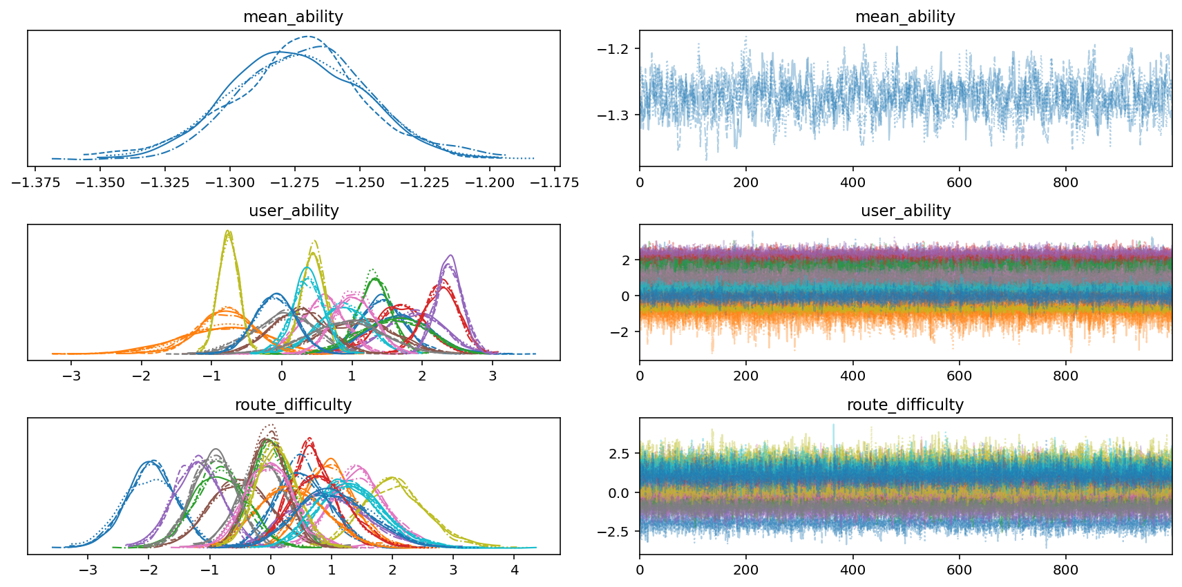
We begin analyzing our modeling outcomes by plotting the MCMC traces. We’ll plot the mean_ability and 20 user_ability and route_difficulty parameters. The hint plots are on the proper, and the density plots (that are like a smoth histogram) are on the left. For the hint plots, educational papers let you know to search for, and I quote, “furry caterpillars”. Our traces look moderately furry and caterpillar-y. For the denisty plots, we will see that our numerous parameters look pretty Gaussian and never too loopy. Looks as if issues are trying OK!
axs = az.plot_trace(
    idata,
    var_names=["mean_ability", "user_ability", "route_difficulty"],
    coords={"user_ability_dim_0": slice(0, 20), "route_difficulty_dim_0": slice(0, 20)},
)


plt.tight_layout()
None
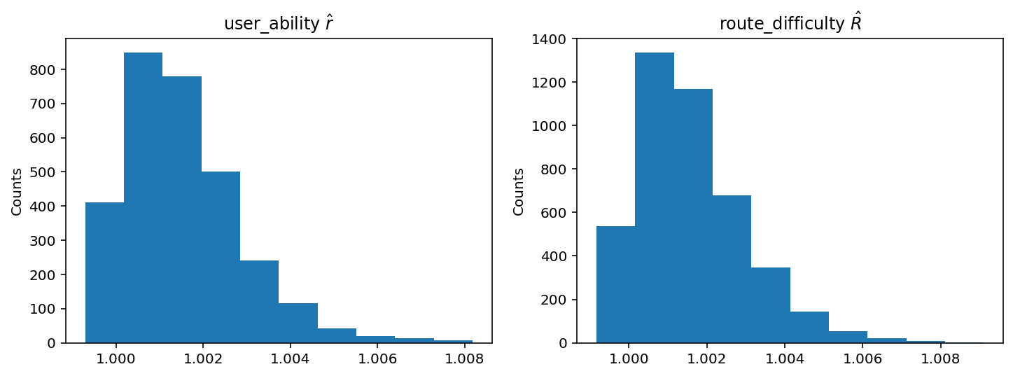
Subsequent, we will examine the notorious $hat{R}$, which is a “convergence diagnostic” for every parameter of the fitted mannequin. The newest analysis says that you really want it to be lower than 1.01. Wanting on the histograms beneath of $hat{R}$ values for user_ability and route_difficulty, it looks like all of them lie beneath 1.01.
fig, axs = plt.subplots(1, 2, figsize=(12, 4))
axs = axs.flatten()
axs[0].hist(model_summary["user_ability"].sel(metric="r_hat").values)
axs[0].set_title("user_ability $hat{r}$")
axs[0].set_ylabel("Counts")
axs[1].hist(model_summary["route_difficulty"].sel(metric="r_hat").values)
axs[1].set_title("route_difficulty $hat{R}$")
axs[1].set_ylabel("Counts")
None
Viz
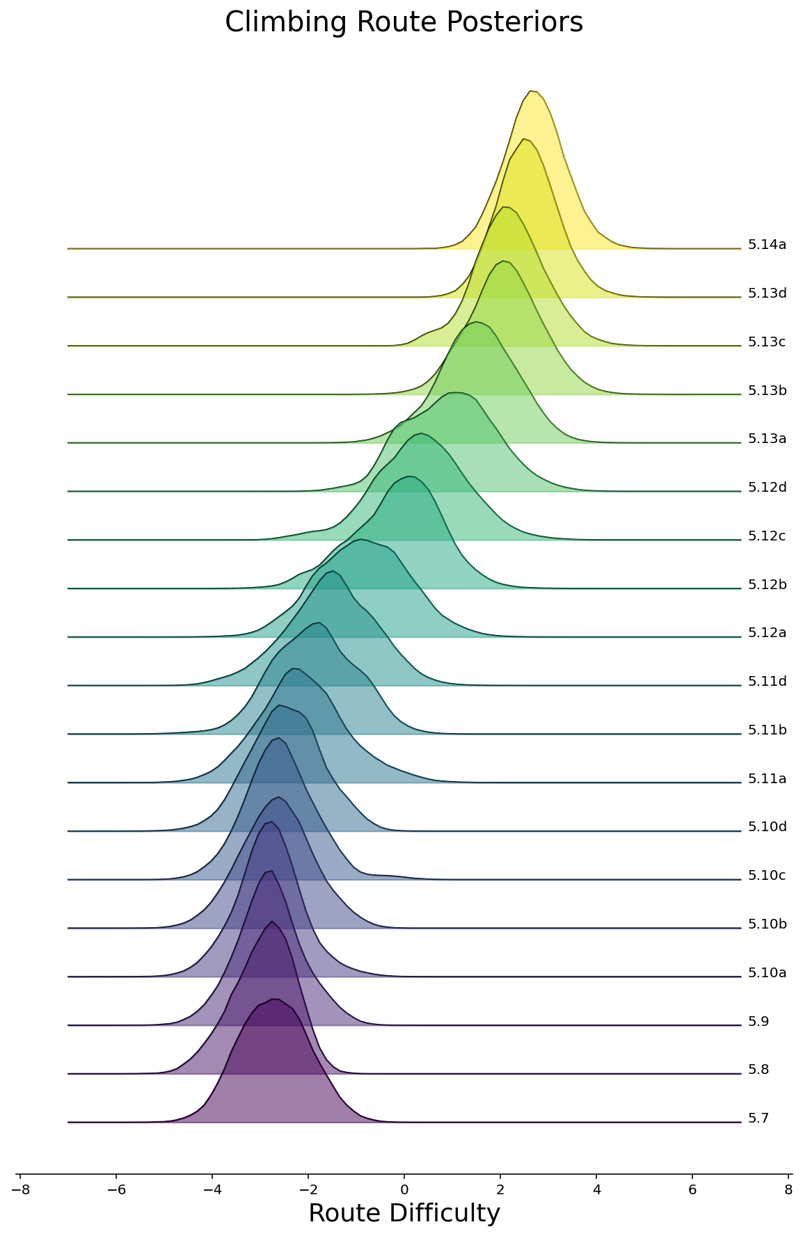
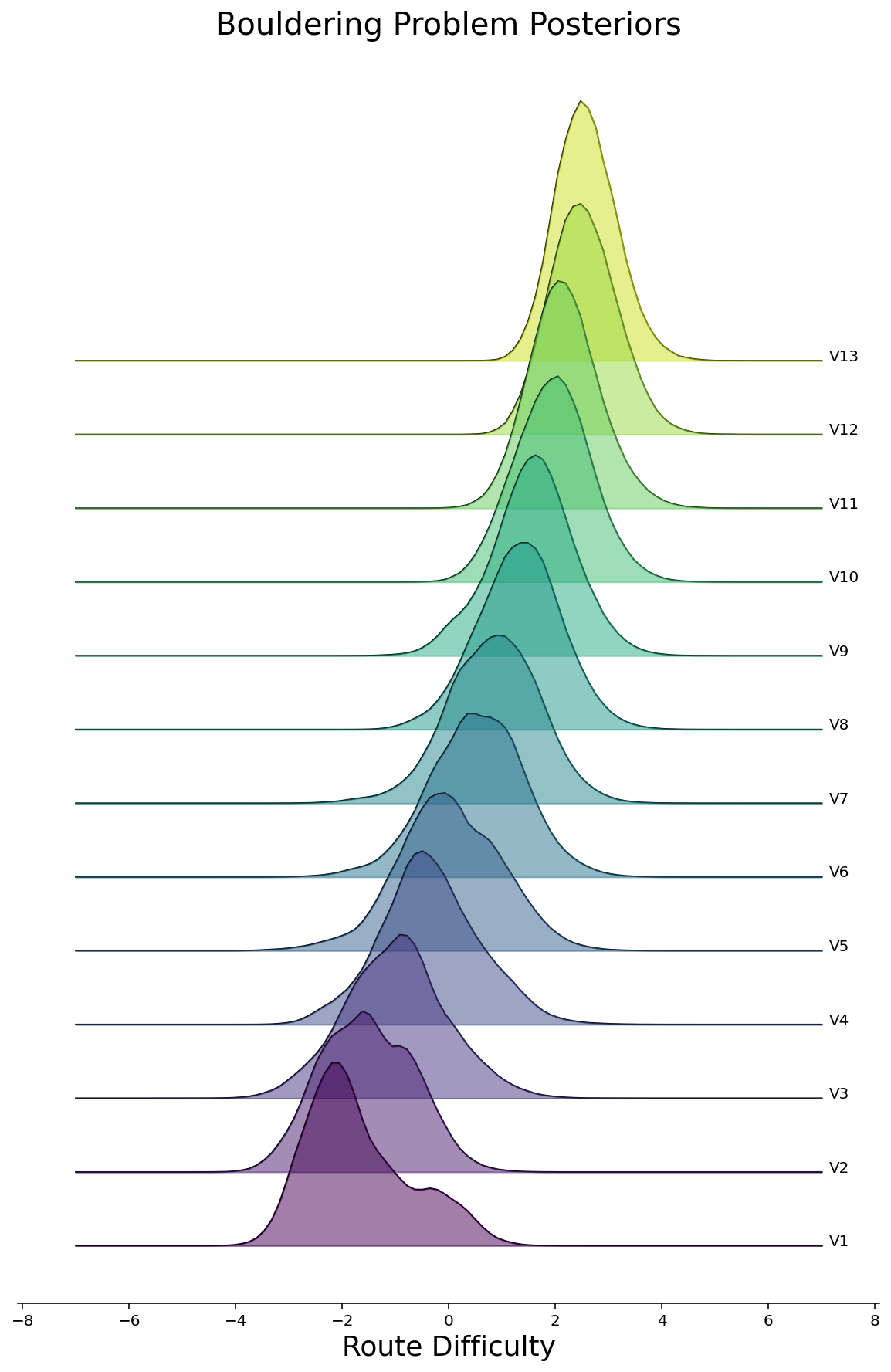
Now that we will really feel considerably comfy that we’ve fitted a halfway-decent mannequin, let’s see what pops out. To start out, we will make density plots of the posteriors for all routes, grouped by the route issue. We’ll do that within the model of a joyplot beneath for Rope and Bouldering routes individually. As we’d hope to see, the posterior difficulties are bigger for routes with larger rankings.
def joyplot(df: pd.DataFrame, routes: pd.DataFrame, rating_col: str, ax=None):
    if ax is None:
        fig, ax = plt.subplots(figsize=(10, 15))

    if rating_col == "route_rating":
        climb_type = 0
    elif rating_col == "bouldering_grade":
        climb_type = 1
    else:
        elevate ValueError(f"Invalid rating_col={rating_col!r}")

    difficulties = df[rating_col].cat.remove_unused_categories().values.classes
    color_map = plt.cm.viridis(np.linspace(0, 1, len(difficulties)))
    ax.set_prop_cycle(cycler.cycler("coloration", color_map))
    total_offset = 0
    delta = 0.2
    num_points = 100
    factors = np.linspace(-7, 7, num_points)
    xmax = 0.0
    zorder = len(difficulties)
    for issue, coloration in zip(difficulties, color_map):
        these_routes = df.loc[
            (df["climb_type"] == climb_type) & (df[rating_col] == issue),
            "route_idx",
        ].distinctive()

        if len(these_routes) > 0:
            these_difficulties = route_difficulties.loc[these_routes].values.ravel()
            kernel = gaussian_kde(these_difficulties)
            density = kernel(factors)
            ax.plot(
                factors,
                density + total_offset,
                coloration="ok",
                linewidth=1,
                label=issue,
                zorder=zorder,
            )
            ax.fill_between(
                factors,
                total_offset,
                density + total_offset,
                coloration=coloration,
                zorder=zorder,
                alpha=0.5,
            )
            x, y = (factors[-1], (density + total_offset)[-1])
            ax.annotate(issue, xy=(x, y), xytext=(1.02 * x, y), coloration="ok")
            total_offset += delta
            zorder -= 1
    xlim = ax.get_xlim()
    ax.set_xlim(xlim[0] * 1.05, xlim[1] * 1.05)
    ax.set_xlabel("Route Problem", fontsize=18)
    ax.spines["right"].set_visible(False)
    ax.spines["top"].set_visible(False)
    ax.spines["left"].set_visible(False)
    ax.set_yticks([])
    ax.set_yticks([], minor=True)
    return ax
route_difficulties = (
    idata["posterior"]["route_difficulty"].to_dataframe().unstack(degree=[0, 1])
)
ax = joyplot(df, route_difficulties, "route_rating")
ax.set_title("Climbing Route Posteriors", fontsize=20)
None
ax = joyplot(df, route_difficulties, "bouldering_grade")
ax.set_title("Bouldering Downside Posteriors", fontsize=20)
None
We are able to discard the total posterior and simply take a look at the imply difficulties for every route. We’ll scatter plot these beneath, once more grouped by ranking. Hovering over every level reveals the title of the climb.
def get_route_difficulties(
    df: pd.DataFrame, climb_type: str, model_summary
) -> pd.DataFrame:
    climb_type_map = {"rope": 0, "boulder": 1}
    if climb_type not in climb_type_map:
        elevate ValueError(f"climb_type should be considered one of {checklist(climb_type.keys())!r}")

    climb_type_ascents = df[df["climb_type"] == climb_type_map[climb_type]]
    routes = climb_type_ascents[
        [
            "route_id",
            "route_idx",
            "crag",
            "route_name",
            "route_rating",
            "bouldering_grade",
        ]
    ].drop_duplicates()

    # Merge difficulties
    # This dataframe is listed by the route_idx
    route_difficulties = model_summary["route_difficulty"].to_dataframe().loc["mean"]

    routes = pd.merge(routes, route_difficulties, left_on="route_idx", right_index=True)
    return routes
def make_stripplot(routes: pd.DataFrame, rating_col: str, title: str):
    rating_order = (
        routes[rating_col]
        .cat.remove_unused_categories()
        .values.classes.tolist()[::-1]
    )

    stripplot = (
        alt.Chart(routes, width=500, top=40, title=title)
        .mark_circle(measurement=50)
        .encode(
            y=alt.Y(
                "jitter:Q",
                title=None,
                axis=alt.Axis(values=[0], ticks=True, grid=False, labels=False),
                scale=alt.Scale(),
            ),
            x=alt.X("route_difficulty:Q", title="Route Problem"),
            coloration=alt.Colour(
                f"{rating_col}:N",
                legend=None,
                scale=alt.Scale(scheme="viridis"),
                type=rating_order,
            ),
            row=alt.Row(
                f"{rating_col}:N",
                title="Score",
                header=alt.Header(
                    labelAngle=0,
                    titleOrient="left",
                    labelOrient="left",
                    labelAlign="left",
                    labelPadding=3,
                ),
                type=rating_order,
            ),
            tooltip=["crag", "route_name"],
        )
        .transform_calculate(
            # Generate Gaussian jitter with a Field-Muller rework
            jitter="sqrt(-2*log(random()))*cos(2*PI*random())"
        )
        .configure_facet(spacing=0)
        .configure_view(stroke=None)
    )

    return stripplot
rope_routes = get_route_difficulties(df, "rope", model_summary)
make_stripplot(rope_routes, "route_rating", "Climbing Route Difficulties")
boulder_routes = get_route_difficulties(df, "boulder", model_summary)
make_stripplot(boulder_routes, "bouldering_grade", "Bouldering Downside Difficulties")
In lieu of truly climbing the routes, we will lookup opinions for routes which have anomalously low or excessive issue for his or her ranking. Pupil Mortgage at Rumney seems to be the toughest 5.11a climb. Wanting the route up on Mountain Undertaking, we will see that they charge it 5.11b, and the outline says:
I’ve heard this route referred to as 5.11a, however I feel its crux is tougher, so I referred to as it 5.11b….
Looks as if our mannequin was proper to charge this a really exhausting 5.11a!
Then again, the best 5.11b is I Simply Do Eyes at Ten Sleep Canyon, and there’s no indication from the opinions on Mountain Undertaking that it is a notably simple route. It’s nearly like our mannequin isn’t excellent.
Our Mannequin is Mistaken
In reality, as I discussed on the prime, our mannequin is most undoubtedly incorrect. There are some apparent indicators: there’s heavy overlap between rankings. For instance, there are some 5.11a climbs which have larger difficulties than some 5.12d climbs. I extremely doubt that that is true, regardless of how subjective the rankings are!
So why is our mannequin incorrect? One evident subject is that we assume user_ability is static whereas folks sometimes get higher at climbing over time. Folks additionally worsen. Keep in mind that pandemic when gyms had been closed?
As talked about earlier than, the information additionally has points. It’d be a lot better to suit an ordinal regression mannequin (as is finished within the Sew Repair publish) to foretell one thing associated to what number of tries it took the person to climb the route (e.g. 1st strive, 2-10, 11+, By no means).The dataset is probably going biased, too. There’s restricted knowledge for simpler climbs, so the difficulties are probably not as well-calibrated. We’re trusting that individuals report their climbs precisely.
However, although all of this was incorrect, I had enjoyable making these plots. If climbing gyms ever began to trace this knowledge, they may extra objectively charge their routes. They might even resolve the “chilly begin ranking” drawback by having a pair folks climb the route after which routinely assign a ranking. Till then, for those who can’t climb the route, then simply inform your self that it’s sandbagged.
